Are you doing parallel computations in R? Then use BiocParallel
It’s the morning of the first day of oral conferences at #ENAR2016. I feel like I have a spidey sense since I woke up 3 min after an email from Jeff Leek; just a funny coincidence. Anyhow, I promised Valerie Obenchain at #Bioc2014 that I would write a post about one of my favorite Bioconductor packages: BiocParallel (Morgan, Obenchain, Lang, and Thompson, 2016). By now it’s on the top 5% of downloaded Bioconductor packages, so many people know about it or are unaware that their favorite package uses it behind the scenes.

While I haven’t blogged about BiocParallel yet, I did give a presentation about it at our computing club back in April 2nd, 2015. See it here (source). I’m going to follow its structure in this post.
Parallel computing
Before even thinking about using BiocParallel you have to decide whether parallel computing is the thing you need.

While I’m not talking about cloud computing, I still find this picture funny.

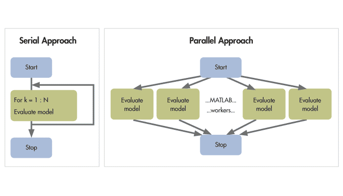
There’s different types of parallel computing, but what I’m referring to here is called embarrassingly parallel where you have a task to do for a set of inputs, you split your inputs into subsets and perform the task on these subsets. Performing this task for one input a a time is called serial programming and it’s what we do in most cases when using functions like lapply() or for loops.
plot(y = 10 / (1:10), 1:10, xlab = 'Number of cores', ylab = 'Time',
    main = 'Ideal scenario', type = 'o', col = 'blue',
    cex = 2, cex.axis = 2, cex.lab = 1.5, cex.main = 2, pch = 16)

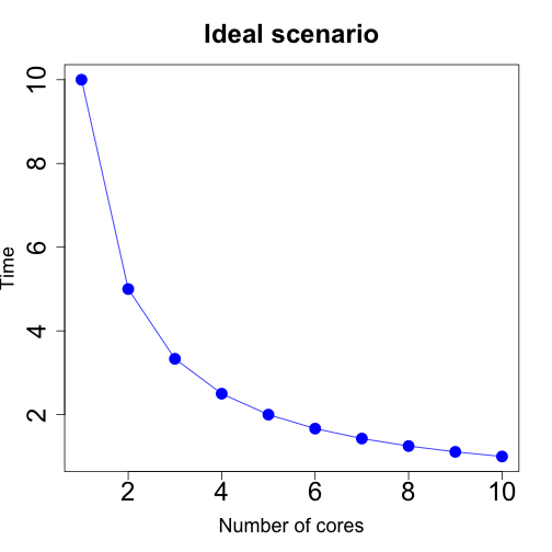
You might be running a simulation for a different set of parameters (a parameter grid) and running each simulation could take some time. Parallel computing can help you speed up this problem. In the ideal scenario, the higher number of computing cores (units that evaluate subsets of your inputs) the less time you need to run your full analysis.
plot(y = 10 / (1:10), 1:10, xlab = 'Number of cores', ylab = 'Time',
    main = 'Reality', type = 'o', col = 'blue',
    cex = 2, cex.axis = 2, cex.lab = 1.5, cex.main = 2, pch = 16)
lines(y = 10 / (1:10) * c(1, 1.05^(2:10) ), 1:10, col = 'red',
    type = 'o', cex = 2)

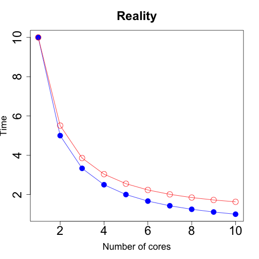
However, in reality parallel computing is not cost-free. It involves some communication costs, like sending the data to the cores, aggregating the results in a way that you can then easily use, among other things. So, it’ll be a bit slower than the ideal scenario but you can potentially still greatly reduce the overall time.
Having said all of the above, lets say that you now want to do some parallel computing in R. Where do you start? A pretty good place to start is the CRAN Task View: High-Performance and Parallel Computing with R. There you’ll find a lot of information about different packages that enable you to do parallel computing with R.

But you’ll soon be lost in a sea of new terms.
Why use BiocParallel?
- It’s simple to use.
- You can try different parallel backends without changing your code.
- You can use it to submit cluster jobs.
- You’ll have access to great support from the Bioconductor developer team.
Those are the big reasons of why I use BiocParallel. But let me go through them a bit more slowly.
Birthday example
I’m going to use as an example the birthday problem where you want to find out empirically the probability that two people share the same birthday in a room.
birthday <- function(n) {
    m <- 10000
    x <- numeric(m)
    for(i in seq_len(m)) {
        b <- sample(seq_len(365), n, replace = TRUE)
        x[i] <- ifelse(length(unique(b)) == n, 0, 1)
    }
    mean(x)
}
Naive birthday code
Once you have written the code for it, you can then use lapply() or a for loop to calculate the results.
system.time( lapply(seq_len(100), birthday) )
##    user  system elapsed
##  25.610   0.442  27.430
Takes around 25 seconds.
Via doMC
If you looked at CRAN Task View: High-Performance and Parallel Computing with R you might have found the doMC (Analytics and Weston, 2015).
It allows you to run computations in parallel as shown below.
library('doMC')
## Loading required package: foreach
## Loading required package: iterators
## Loading required package: parallel
registerDoMC(2)
system.time( x <- foreach(j = seq_len(100)) %dopar% birthday(j) )
##    user  system elapsed
##  12.819   0.246  13.309
While it’s a bit faster, the main problem is that you had to change your code in order to be able to use it.
With BiocParallel
This is how you would run things with BiocParallel.
library('BiocParallel')
system.time( y <- bplapply(seq_len(100), birthday) )
##    user  system elapsed
##   0.021   0.011  16.095
The only change here is using bplapply() instead of lapply(), so just 2 characters. Well, that and loading the BiocParallel package.
BiocParallel’s advantages
There are many computation backends and one of the strongest features of BiocParallel is that it’s easy to switch between them. For example, my computer can run the following options:
registered()
## $MulticoreParam
## class: MulticoreParam
##   bpjobname:BPJOB; bpworkers:2; bptasks:0; bptimeout:Inf; bpRNGseed:; bpisup:FALSE
##   bplog:FALSE; bpthreshold:INFO; bplogdir:NA
##   bpstopOnError:FALSE; bpprogressbar:FALSE
##   bpresultdir:NA
## cluster type: FORK
##
## $SnowParam
## class: SnowParam
##   bpjobname:BPJOB; bpworkers:2; bptasks:0; bptimeout:Inf; bpRNGseed:; bpisup:FALSE
##   bplog:FALSE; bpthreshold:INFO; bplogdir:NA
##   bpstopOnError:FALSE; bpprogressbar:FALSE
##   bpresultdir:NA
## cluster type: SOCK
##
## $SerialParam
## class: SerialParam
##   bplog:FALSE; bpthreshold:INFO
##   bpcatchErrors:FALSE
If I was doing this in our computing cluster, I would see even more options.
Now lets say that I want to test different computation backends, or even run things in serial mode so I can trace a bug down more easily. Well, all I have to do is change the BPPARAM argument as shown below.
## Test in serial mode
system.time( y.serial <- bplapply(1:10, birthday,
    BPPARAM = SerialParam()) )
##    user  system elapsed
##   2.577   0.033   2.733
## Try Snow
system.time( y.snow <- bplapply(1:10, birthday,
    BPPARAM = SnowParam(workers = 2)) )
##    user  system elapsed
##   0.027   0.006   2.436
Talking about computing clusters, you might be interested in using BatchJobs (Bischl, Lang, Mersmann, Rahnenführer, et al., 2015) just like Prasad Patil did for his PhD work. Well, with BiocParallel you can also chose to use the BatchJobs backend. I have code showing this at the presentation I referenced earlier.
Where do I start?
If you are convinced about using BiocParallel, which I hope you are by now, check out the Introduction to BiocParallel vignette available at BiocParallel’s landing page. It explains in more detail how to use it and it’s rich set of features. But if you just want to jump right in and start playing around with it, install it by running the following code:
install.packages("BiocManager")
BiocManager::install("BiocParallel")
Conclusions
Like I said earlier, BiocParallel is simple to use and has definite advantages over other solutions.
- You can try different parallel backends without changing your code.
- You can use it to submit cluster jobs.
- You’ll have access to great support from the Bioconductor developer team. See the biocparallel tag at the support website.
Have fun using it!
Reproducibility
## Reproducibility info
library('devtools')
session_info()
## Session info --------------------------------------------------------------
##  setting  value
##  version  R version 3.2.2 (2015-08-14)
##  system   x86_64, darwin13.4.0
##  ui       X11
##  language (EN)
##  collate  en_US.UTF-8
##  tz       America/Chicago
##  date     2016-03-07
## Packages ------------------------------------------------------------------
##  package        * version  date       source
##  bibtex           0.4.0    2014-12-31 CRAN (R 3.2.0)
##  BiocParallel   * 1.4.3    2015-12-16 Bioconductor
##  bitops           1.0-6    2013-08-17 CRAN (R 3.2.0)
##  codetools        0.2-14   2015-07-15 CRAN (R 3.2.2)
##  devtools       * 1.10.0   2016-01-23 CRAN (R 3.2.3)
##  digest           0.6.9    2016-01-08 CRAN (R 3.2.3)
##  doMC           * 1.3.4    2015-10-13 CRAN (R 3.2.0)
##  evaluate         0.8      2015-09-18 CRAN (R 3.2.0)
##  foreach        * 1.4.3    2015-10-13 CRAN (R 3.2.0)
##  formatR          1.2.1    2015-09-18 CRAN (R 3.2.0)
##  futile.logger    1.4.1    2015-04-20 CRAN (R 3.2.0)
##  futile.options   1.0.0    2010-04-06 CRAN (R 3.2.0)
##  httr             1.1.0    2016-01-28 CRAN (R 3.2.3)
##  iterators      * 1.0.8    2015-10-13 CRAN (R 3.2.0)
##  knitcitations  * 1.0.7    2015-10-28 CRAN (R 3.2.0)
##  knitr          * 1.12.3   2016-01-22 CRAN (R 3.2.3)
##  lambda.r         1.1.7    2015-03-20 CRAN (R 3.2.0)
##  lubridate        1.5.0    2015-12-03 CRAN (R 3.2.3)
##  magrittr         1.5      2014-11-22 CRAN (R 3.2.0)
##  memoise          1.0.0    2016-01-29 CRAN (R 3.2.3)
##  plyr             1.8.3    2015-06-12 CRAN (R 3.2.1)
##  R6               2.1.2    2016-01-26 CRAN (R 3.2.3)
##  Rcpp             0.12.3   2016-01-10 CRAN (R 3.2.3)
##  RCurl            1.95-4.7 2015-06-30 CRAN (R 3.2.1)
##  RefManageR       0.10.6   2016-02-15 CRAN (R 3.2.3)
##  RJSONIO          1.3-0    2014-07-28 CRAN (R 3.2.0)
##  snow             0.4-1    2015-10-31 CRAN (R 3.2.0)
##  stringi          1.0-1    2015-10-22 CRAN (R 3.2.0)
##  stringr          1.0.0    2015-04-30 CRAN (R 3.2.0)
##  XML              3.98-1.3 2015-06-30 CRAN (R 3.2.0)
References
Citations made with knitcitations (Boettiger, 2015).
[1] R. Analytics and S. Weston. doMC: Foreach Parallel Adaptor for 'parallel'. R package version 1.3.4. 2015. URL: http://CRAN.R-project.org/package=doMC.
[2] B. Bischl, M. Lang, O. Mersmann, J. Rahnenführer, et al. “BatchJobs and BatchExperiments: Abstraction Mechanisms for Using R in Batch Environments”. In: Journal of Statistical Software 64.11 (2015), pp. 1–25. URL: http://www.jstatsoft.org/v64/i11/.
[3] C. Boettiger. knitcitations: Citations for 'Knitr' Markdown Files. R package version 1.0.7. 2015. URL: http://CRAN.R-project.org/package=knitcitations.
[4] M. Morgan, V. Obenchain, M. Lang and R. Thompson. BiocParallel: Bioconductor facilities for parallel evaluation. R package version 1.4.3. 2016.
Want more?
Check other @jhubiostat student blogs at Bmore Biostats as well as topics on #rstats.