Teaching omics methods to LCG-UNAM students

Valentina Arias Ojeda is as teaching assistant for the class “Omics Research Techniques”, taught by Dr. Constance Auvynet at LCG-UNAM. They invited me to teach a class on single cell RNA-seq and spatially-resolved transcriptomics. Valentina introduced me and then I mentioned a bit of my teaching history, starting from my first teaching experience where I made a website available in both English and Spanish.

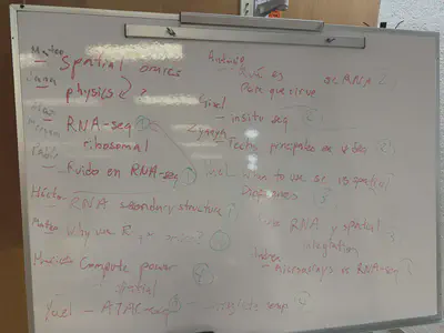
I decided to teach today’s class as a collective “Data Science guidance session”. However, unlike a regular DSgs, we first needed to come up with a list of questions or concepts that they wanted to learn more about. Here I used a technique I learned as a teaching assistant for the 140.620 series on Statistical Methods in Public Health at JHU. That is, write on the board the questions, then try to group them up into different categories. Our full list of questions was:

1. RNA-seq
   • What is the difference between microarrays and RNA-seq?
   • What is RNA-seq?
   • How do we deal with ribosomal RNAs in RNA-seq?
   • How do we deal with noise in RNA-seq?
     • How do we define noise?
   • How does RNA-seq deal with RNA secondary structures?
2. Single cell RNA-seq
   • What is scRNA-seq?
   • What is scRNA-seq useful for?
   • Which are the main sequencing technologies?
   • What is ATAC-seq?
   • What is insitu seq?
3. Spatially resolved transcriptomics
   • What is spatially resolved transcriptomics?
   • What is the difference between spatially resolved transcriptomics and scRNA-seq?
   • How can we integrate RNA-seq and spatially resolved transcriptomics?
   • What are the physics behind spatially resolved transcriptomics?
4. Data analysis
   • Why do we use R for omics data analysis?
     • How do we analyze RNA-seq data?
     • How do we analyze scRNA-seq data?
     • How do we analyze spatially resolved transcriptomics data?
   • How much computational power do we need for spatial omics data analysis?
   • How do we integrate RNA-seq and spatially resolved transcriptomics data?

RNA-seq

I used this slide with an image from Gandal et al DOI 10.1016/j.biopsych.2020.06.005 that shows many types of RNA molecules. Many are mostly interested in mRNA: messenger RNA. Though other RNA molecules can be of interest, such as microRNAs.

For microarrays, I explained how they are probe-based assays where a company designs the probes, prints them on a glass screen, and how the data is generated through high resolution images (photos) of the glass screen. To do this, you have to know the gene annotation (where genes are located in the genome) in order to design the probes. Microarrays are cheaper than RNA-seq and have been used a lot for DNA genotyping, where we are interested in a set of 2.5 million or so locations in the genome that commonly vary between individuals.

RNA-seq really came to be popular or well, possible, with the advent of next generation sequencing. The idea is that you can sequence the RNA molecules in a sample and then align the sequences to the genome to know where they came from. This is more expensive than microarrays but it has the advantage that you don’t need to know the gene annotation beforehand. This is because you can align the sequences to the genome and then count how many sequences align to each gene. You can also study isoforms (transcripts), instead of genes. A quick Google search led me here as I wanted to show them an illustration of a gene with multiple transcripts, some of them with very small differences between them. We also looked at Gencode’s release history to highlight that the gene annotation is not static and frequently updated.

For a quick intro to next generation sequencing or high-throughput sequencing (these were synonyms in 2006 to 2011 or so), I went back to a course I taught for UNAM PhD students shortly after finishing my undergrad. From https://lcolladotor.github.io/courses/PDCB-HTS.html, we looked at the slide deck for “2. Understanding the technology”. Particularly slides 39 to 42 where I briefly explained Illumina short read sequencing.

In relation to ribosomal RNAs, I explained the two most common RNA-seq protocols: polyA+ and ribo-depletion (RiboZeroGold). I used a preprint we wrote in 2024 where Figure 1B shows the two RNA-seq library types but also the different RNA extraction protocols (often something people ignore).

Figure 1D highlights how different the data using principal components (PC1 separates library type, PC2 separates RNA extractions), and Figure 1E shows within a given RNA extraction, how genes are differentially quantified by the two library types.

For noise in RNA-seq, we looked at my derfinder PhD paper. Figure 1 actually is a reminder of how transcripts can have very small differences between them. Figure 2 has coverage curves for RNA-seq data. We used derfinder when we studied human brain expression changes across age groups including prenatal samples DOI 10.1038/nn.3898. Through that work we concluded that the human brain transcriptome was incomplete. I mentioned also how polyA and RiboZeroGold data will have different coverage profiles (RiboZeroGold will show coverage for introns as some pre-mRNAs are going to be sequenced). I also described the totalAssignedGene metric that SPEAQeasy generates: the fraction of reads assigned to genes from the total number of reads that were aligned to the genome. We’ve used totalAssignedGene to identify poor quality samples in some studies.

I also briefly mentioned that an advantage of RNA-seq is the possibility of assembling transcripts using tools like StringTie developed by some of my collaborators. They ran StringTie on the ~10,000 GTEx RNA-seq samples to build CHESS. Eventually from ~26 million transcripts they filtered the list and found ~160,000 transcripts DOI 10.1186/s13059-023-03088-4. There are many challenges on how you decide what is a real transcript versus noise. Do you trust more a transcript with 100 reads but only in one sample or a transcript with 5 reads per sample that is present in 10% of your samples?

As for secondary structures in RNA, I explained how RNA-seq protocols involve a step where RNA is cut into fragments of about 300 to 500 base pairs. That’s one way to deal with RNA secondary structures. Though I don’t remember if there are other steps that help avoid issues with RNA tangling. And it might be something that we forget about: some RNAs that are more likely to fold might not be as well represented in RNA-seq data.

scRNA-seq

For scRNA-seq, I used parts of this explanatory video from 10x Genomics. I paused it a few times to highlight the GEMs, the fluidics for getting cells into droplets, and how each droplet has a cell barcode (a unique DNA sequence), and there’s about 750,000 of them on a given experiment.

In the end you generate DNA that you can sequence with Illumina sequencers. Actually, many other protocols are all about generating DNA for the molecules of interest, then sequencing those DNA molecules with Illumina. For example, ChIP-seq, ATAC-seq, etc.

Spatially resolved transcriptomics

To explain spatially-resolved transcriptomics, I showed the students my blog post (with English and Spanish videos) explaining the first 10x Genomics Visium paper which we wrote DOI 10.1038/s41593-020-00787-0. I highlighted how Visium uses “spatial barcodes”, akin to the scRNA-seq barcodes we saw previously. These DNA sequences label the nearly 5,000 spots present on a Visium slide. Here’s a short 10x Genomics intro to Visium video.

For the tissue we were studying (human brain DLPFC), we found that each Visium spot contained on average 3 cells. With spatial omics you find how cells are grouped spatially, which can be informative unlike what we obtain with scRNA-seq (individual cell expression profiles with no spatial information) or bulk RNA-seq (like blending together a bunch of cells and getting the overall mean expression profile). Spot deconvolution, which we benchmarked a bit at DOI 10.1126/science.adh1938, and bulk RNA-seq deconvolution which we’ve also benchmarked at DOI 10.1101/2024.02.09.579665, are some computational methods that allow integrating multiple flavors of RNA-seq together. Dai et al also wrote a really nice benchmark paper for second generation bulk RNA-seq deconvolution methods using scRNA-seq data as the reference: DOI 10.1126/sciadv.adh2588.

I also highlighted how with bulk RNA-seq some LIBD datasets have 80 million paired-end reads of 100 base-pairs each (as about $1,000 USD per sample). Ultimately, the read length (in base pairs) multiplied by the number of reads determines how much money you are doing to spend sequencing. 10x Genomics recommends 50,000 reads per cell for scRNA-seq or per spot for Visium. A Visium capture area has 5,000 spots, aka, that’s 250 million reads per Visium capture area. You do spend about 2,000 to 2,500 USD per Visium capture area just for Illumina sequencing without including other 10x Genomics reagents. Also, the options you have per cell or per spot are limited as you went from 80 million reads to 50 thousand (a 1,600x reduction!). So scRNA-seq and Visium are much more sparse than bulk RNA-seq. Some scRNA-seq protocols are also 3’ biased, meaning that you only sequence the 3’ end of the RNA molecules. Some have developed ways of quantifying transcripts despited these biases, but it’s still an active area of research. Overall though, the data generation costs for each assay sometimes determines what assays one can use. However, if others have shared relevant data, then you can re-use that data and don’t have to generate all yourself.

In terms of the best methods for RNA-seq sequencing and associated assays, I mentioned that one way to check this is by looking at the valuation of these companies and their stock prices. These companies frequently acquire smaller companies, sue each other, etc. Some of them have been impacted by recent trade wars, for example China bans imports of Illumina’s gene sequencers right after Trump tariff action. This was partially done because two genomics Chinese companies were accused by the US on grounds of national security. Overall, Illumina and 10x Genomics are among the biggest players in the field. There are other large companies, and many small ones (20 or so employees), some of which aim to be acquired by the big ones.

Data Analysis

I’ll see these same second semester students a year from now when they take the fourth semester class on introduction to RNA-seq data analysis with R and Bioconductor that I’ve taught the last five years. As a quick teaser, I mentioned that Bioconductor is a great repository of open source software for the analysis of high throughput biological data: microrrays 23 or so years ago and nowdays scRNA-seq and spatial omics. It’s also mandatory to write user guides (vignette documents) on all Bioconductor software. This makes it much easier to learn how to use the software and it’s a distinctive factor that separates Bioconductor from other software repositories.

From my team’s recent TL DR (too long, did not read) presentation I showed a few slides.

Check our recent video "[2025-01-29] R/Bioconductor-powered Team Data Science: TLDR version 2025" youtu.be/alL-g2roXxM

We go over what analyses our @lieberinstitute.bsky.social has expertise on 💻

Slides orchestrated by @lahuuki.bsky.social at speakerdeck.com/lahuuki/2025…

👥 go.bsky.app/53gy4UP

[image or embed]

— 🇲🇽 Leonardo Collado-Torres (@lcolladotor.bsky.social) February 12, 2025 at 3:35 PM

First I showed how Visium HD is a new technlogy from 10x Genomics that is probe based. So think about it as a modern microarray that is spatially-resolved. It’s also powered enough to generate sub-cellular resolution data: starting at 2 micron squares.

Analyzing that data can be computationally demanding in terms of requiring GPUs and/or high-memory compute nodes.

Ultimately, there can be a need to uniformly process publicly available RNA-seq data to democratize access to this data such that researchers without access to high performant compute environments are also able to analyze these valuable datasets. I worked on this through the recount2 and recount3 DOI 10.1186/s13059-021-02533-6 projects. I’ll teach them more about this next year.

Miscellaneous

I ended with highlighting the resources from the Community of Bioinformatics Software Developers (CDSB in Spanish) and the LIBD RStats Club. There students can find videos from full week-long workshops such as the 2021 scRNA-seq analysis course and many other videos from LIBD RStats Club schedule.

I also highlighted how one has to spend work hours trying to learn new methods instead of relying on doing so on your free time. Finally, I highlighted how I like to learn in public. How sharing what you know can be helpful not just to others, but yourself.

It’s always great to be back at LCG-UNAM, my undergrad alma mater. I also enjoy interacting with current students. Here I’m with Valentina and Bernardo, both of whom are working as teaching assistants and finishing their third year. Next up is their final year which is a research year. I’m looking forward to learning about that they end up choosing to work on and to witness their careers flourish.