This lecture, as the rest of the course, is adapted from the version Stephanie C. Hicks designed and maintained in 2021 and 2022. Check the recent changes to this file through the GitHub history.

Interacting with LLMs in RStudio IDE / Positron

Can we use ChatGPT or other LLMs to help us write R code in this class?

Or what about outside of this class? After all, it’ll be done sooner rather than later.

Yes you can! Though I think that using GitHub Copilot is likely the most efficient option, I want to highlight a new package called chattr that allows you to use LLMs like GPT-4.1 directly from RStudio IDE / Positron. chattr is documented at https://mlverse.github.io/chattr/. At this point, hopefully your application to use GitHub Copilot has been approved. If you haven’t completed this application, see our first lecture for the details.

In general, you might want to follow the news from the Posit AI newsletter which was launched last month: https://posit.co/blog/2025-08-29-ai-newsletter/. You might want to follow both Simon P. Couch and Sara Altman on Bluesky or on LinkedIn: Simon P. Couch and Sara Altman.

Below is a demo of how to use chattr with the GitHub Copilot LLM model.

## Install ellmer and chattr
install.packages(c("ellmer", "chattr"))

## Load both packages
library("ellmer")
library("chattr")

## Specify that you'll use the GitHub Copilot model
my_chat <- ellmer::chat_github()
chattr::chattr_use(my_chat)

## Load some packages for analysis
library("tidyverse")

## Load the penguins dataset to have something we can
## explore with
library("palmerpenguins")
glimpse(penguins)

## You can now either interact with the LLM through
## commands like this one:
my_chat$chat("Explore the relationship between bill_length_mm and bill_depth_mm across species and island using ggplot2 color aesthetics and facets.")
my_chat$chat("What do we know the variables in the penguins dataset?")
my_chat$chat("Please provide me a more detailed description and code for exploring this dataset")

## or launch the chattr app
chattr::chattr_app()

## Edit the option to include at least 1 data frame.
## Then type the following prompt:
## Explore the relationship between bill_length_mm and bill_depth_mm across species and island using ggplot2 color aesthetics and facets.

## This was my answer by the gpt-4.1 model:
library(tidyverse)
penguins <- readr::read_csv('https://raw.githubusercontent.com/allisonhorst/palmerpenguins/master/inst/extdata/penguins.csv')

ggplot(penguins, aes(x = bill_length_mm, y = bill_depth_mm, color = species)) +
  geom_point(na.rm = TRUE) +
  facet_wrap(~ island) +
  theme_minimal()
## Notice how it used a "theme_minimal()" although I didn't ask for it!

## If you open the chattr chat again, you'll see 
## your full chat history there too. Now you can
## use the option to also send your chat history
## when sending prompts to the LLM.

## Try:
## Now make the graph interactive using plotly.

## Here was my answer from the LLM:
library(tidyverse)
library(plotly)

penguins <- readr::read_csv('https://raw.githubusercontent.com/allisonhorst/palmerpenguins/master/inst/extdata/penguins.csv')

p <- ggplot(penguins, aes(x = bill_length_mm, y = bill_depth_mm, color = species)) +
  geom_point(na.rm = TRUE) +
  facet_wrap(~ island) +
  theme_minimal()

ggplotly(p)

See chattr::chatter_defaults() for more options on how to customize your experience with chattr https://mlverse.github.io/chattr/reference/chattr_defaults.html.

For more about AI and R, you might want to check the LIBD RStats club 2025-01-31 session on “R coding using GitHub Copilot with RStudio and related R packages”.

Pre-lecture materials

Read ahead

Before class, you can prepare by reading the following materials:

Acknowledgements

Material for this lecture was borrowed and adopted from

https://rdpeng.github.io/Biostat776/lecture-r-nuts-and-bolts

Learning objectives

At the end of this lesson you will:

Know the 5 basic built-in data types (or classes) of objects in R
Know the types of attributes (or metadata) R objects can have
Be able to create a vector, matrix, data frame, factor, and list in R
Recognize missing values in R

R Nuts and Bolts

Entering Input

At the R prompt we type expressions. The <- symbol is the assignment operator.

x <- 1
print(x)

[1] 1

[1] 1

msg <- "hello"

The grammar of the language determines whether an expression is complete or not.

x <-  ## Incomplete expression

Error in parse(text = input): <text>:2:0: unexpected end of input
1: x <-  ## Incomplete expression
   ^

The # character indicates a comment.

Anything to the right of the # (including the # itself) is ignored. This is the only comment character in R.

Unlike some other languages, R does not support multi-line comments or comment blocks.

Evaluation

When a complete expression is entered at the prompt, it is evaluated and the result of the evaluated expression is returned.

The result may be auto-printed.

x <- 5  ## nothing printed
x       ## auto-printing occurs

[1] 5

print(x)  ## explicit printing

[1] 5

The [1] shown in the output indicates that x is a vector and 5 is its first element.

Typically with interactive work, we do not explicitly print objects with the print() function; it is much easier to just auto-print them by typing the name of the object and hitting return/enter.

However, when writing scripts, functions, or longer programs, there is sometimes a need to explicitly print objects because auto-printing does not work in those settings.

When an R vector is printed you will notice that an index for the vector is printed in square brackets [] on the side. For example, see this integer sequence of length 20.

x <- 11:30
x

 [1] 11 12 13 14 15 16 17 18 19 20 21 22
[13] 23 24 25 26 27 28 29 30

The numbers in the square brackets are not part of the vector itself, they are merely part of the printed output.

Note

With R, it’s important that one understand that there is a difference between the actual R object and the manner in which that R object is printed to the console.

Often, the printed output may have additional bells and whistles to make the output more friendly to the users. However, these bells and whistles are not inherently part of the object.

Pro-tip

The : operator is used to create integer sequences.

5:0

[1] 5 4 3 2 1 0

-15:15

 [1] -15 -14 -13 -12 -11 -10  -9  -8  -7  -6  -5  -4  -3  -2  -1   0   1   2   3
[20]   4   5   6   7   8   9  10  11  12  13  14  15

R Objects

The most basic type of R object is a vector.

Vectors

There is really only one rule about vectors in R, which is that

A vector can only contain objects of the same class

To understand what we mean here, we need to dig a little deeper. We will come back this in just a minute.

Types of vectors

There are two types of vectors in R:

Atomic vectors:
- logical: FALSE, TRUE, and NA
- integer (and doubles): these are known collectively as numeric vectors (or real numbers)
- complex: complex numbers
- character: the most complex type of atomic vector, because each element of a character vector is a string, and a string can contain an arbitrary amount of data
- raw: used to store fixed-length sequences of bytes. These are not commonly used directly in data analysis and I won’t cover them here.
Lists, which are sometimes called recursive vectors because lists can contain other lists.

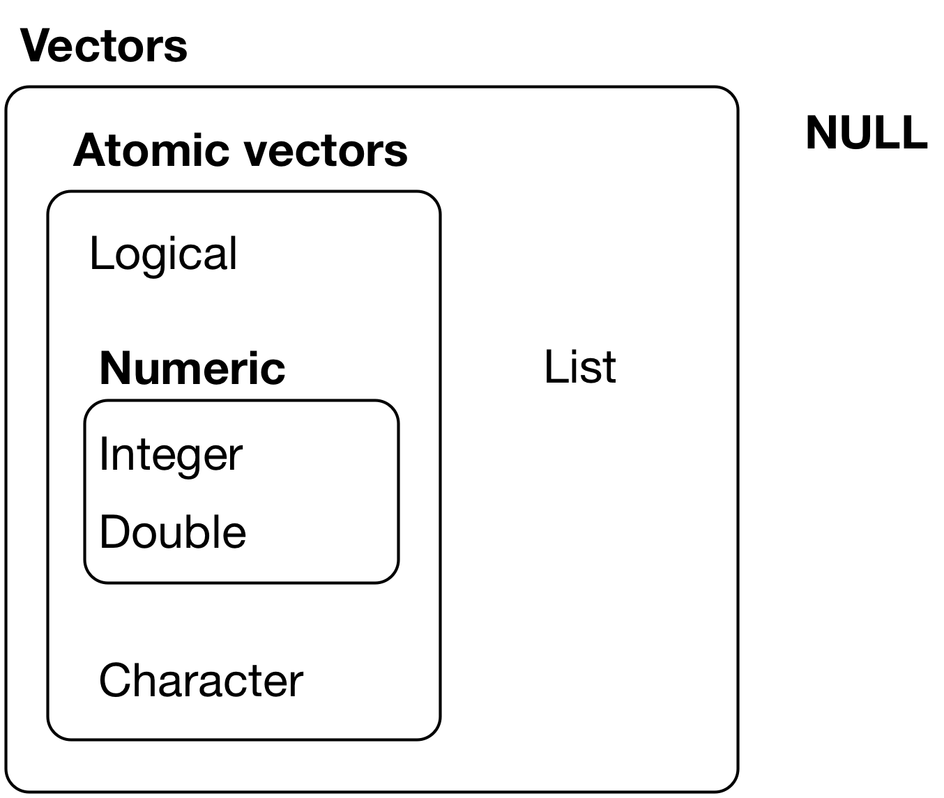
[Source: R 4 Data Science]

Note

There’s one other related object: NULL.

NULL is often used to represent the absence of a vector (as opposed to NA which is used to represent the absence of a value in a vector).
NULL typically behaves like a vector of length 0.

Create an empty vector

Empty vectors can be created with the vector() function.

vector(mode = "numeric", length = 4)

[1] 0 0 0 0

vector(mode = "logical", length = 4)

[1] FALSE FALSE FALSE FALSE

vector(mode = "character", length = 4)

[1] "" "" "" ""

Creating a non-empty vector

The c() function can be used to create vectors of objects by concatenating things together.

x <- c(0.5, 0.6)       ## numeric
x <- c(TRUE, FALSE)    ## logical
x <- c(T, F)           ## logical
x <- c("a", "b", "c")  ## character
x <- 9:29              ## integer
x <- c(1+0i, 2+4i)     ## complex

Note

In the above example, T and F are short-hand ways to specify TRUE and FALSE.

However, in general, one should try to use the explicit TRUE and FALSE values when indicating logical values.

The T and F values are primarily there for when you’re feeling lazy.

Lists

So, I know I said there is one rule about vectors:

A vector can only contain objects of the same class

But of course, like any good rule, there is an exception, which is a list (which we will get to in greater details a bit later).

For now, just know a list is represented as a vector but can contain objects of different classes. Indeed, that’s usually why we use them.

Note

The main difference between atomic vectors and lists is that atomic vectors are homogeneous, while lists can be heterogeneous.

Numerics

Integer and double vectors are known collectively as numeric vectors.

In R, numbers are doubles by default.

To make an integer, place an L after the number:

typeof(4)

[1] "double"

typeof(4L)

[1] "integer"

Note

The distinction between integers and doubles is not usually important, but there are two important differences that you should be aware of:

Doubles are approximations!
Doubles represent floating point numbers that can not always be precisely represented with a fixed amount of memory. This means that you should consider all doubles to be approximations.

Question

Let’s explore this. What is square of the square root of two? i.e. \((\sqrt{2})^2\)

x <- sqrt(2) ^ 2
x

[1] 2

Try subtracting 2 from x? What happened?

## try it here

Numbers

Numbers in R are generally treated as numeric objects (i.e. double precision real numbers).

This means that even if you see a number like “1” or “2” in R, which you might think of as integers, they are likely represented behind the scenes as numeric objects (so something like “1.00” or “2.00”).

This isn’t important most of the time…except when it is!

If you explicitly want an integer, you need to specify the L suffix. So entering 1 in R gives you a numeric object; entering 1L explicitly gives you an integer object.

Note

There is also a special number Inf which represents infinity. This allows us to represent entities like 1 / 0. This way, Inf can be used in ordinary calculations; e.g. 1 / Inf is 0.

The value NaN represents an undefined value (“not a number”); e.g. 0 / 0; NaN can also be thought of as a missing value (more on that later)

Attributes

R objects can have attributes, which are like metadata for the object.

These metadata can be very useful in that they help to describe the object.

For example, column names on a data frame help to tell us what data are contained in each of the columns. Some examples of R object attributes are

names, dimnames
dimensions (e.g. matrices, arrays)
class (e.g. integer, numeric)
length
other user-defined attributes/metadata

Attributes of an object (if any) can be accessed using the attributes() function. Not all R objects contain attributes, in which case the attributes() function returns NULL.

However, every vector has two key properties:

Its type, which you can determine with typeof().

letters

 [1] "a" "b" "c" "d" "e" "f" "g" "h" "i" "j" "k" "l" "m" "n" "o" "p" "q" "r" "s"
[20] "t" "u" "v" "w" "x" "y" "z"

typeof(letters)

[1] "character"

1:10

 [1]  1  2  3  4  5  6  7  8  9 10

typeof(1:10)

[1] "integer"

Its length, which you can determine with length().

x <- list("a", "b", 1:10)
x

[[1]]
[1] "a"

[[2]]
[1] "b"

[[3]]
 [1]  1  2  3  4  5  6  7  8  9 10

length(x)

[1] 3

typeof(x)

[1] "list"

attributes(x)

NULL

Mixing Objects

There are occasions when different classes of R objects get mixed together.

Sometimes this happens by accident but it can also happen on purpose.

Question

Let’s use typeof() to ask what happens when we mix different classes of R objects together.

y <- c(1.7, "a")
y <- c(TRUE, 2)
y <- c("a", TRUE)

## try it here

Why is this happening?

In each case above, we are mixing objects of two different classes in a vector.

But remember that the only rule about vectors says this is not allowed?

When different objects are mixed in a vector, coercion occurs so that every element in the vector is of the same class.

In the example above, we see the effect of implicit coercion.

What R tries to do is find a way to represent all of the objects in the vector in a reasonable fashion. Sometimes this does exactly what you want and…sometimes not.

For example, combining a numeric object with a character object will create a character vector, because numbers can usually be easily represented as strings.

Explicit Coercion

Objects can be explicitly coerced from one class to another using the as.*() functions, if available.

x <- 0:6
class(x)

[1] "integer"

as.numeric(x)

[1] 0 1 2 3 4 5 6

as.logical(x)

[1] FALSE  TRUE  TRUE  TRUE  TRUE  TRUE  TRUE

as.character(x)

[1] "0" "1" "2" "3" "4" "5" "6"

Sometimes, R can’t figure out how to coerce an object and this can result in NAs being produced.

x <- c("a", "b", "c")
as.numeric(x)

Warning: NAs introduced by coercion

[1] NA NA NA

as.logical(x)

[1] NA NA NA

Question

Let’s try to convert the x vector above into integers.

## try it here

When nonsensical coercion takes place, you will usually get a warning from R.

Matrices

Matrices are vectors with a dimension attribute.

The dimension attribute is itself an integer vector of length 2 (number of rows, number of columns)

m <- matrix(nrow = 2, ncol = 3) 
m

     [,1] [,2] [,3]
[1,]   NA   NA   NA
[2,]   NA   NA   NA

dim(m)

[1] 2 3

attributes(m)

$dim
[1] 2 3

Matrices are constructed column-wise, so entries can be thought of starting in the “upper left” corner and running down the columns.

m <- matrix(1:6, nrow = 2, ncol = 3) 
m

     [,1] [,2] [,3]
[1,]    1    3    5
[2,]    2    4    6

Question

Let’s try to use attributes() function to look at the attributes of the m object

## try it here

Matrices can also be created directly from vectors by adding a dimension attribute.

m <- 1:10 
m

 [1]  1  2  3  4  5  6  7  8  9 10

dim(m) <- c(2, 5)
m

     [,1] [,2] [,3] [,4] [,5]
[1,]    1    3    5    7    9
[2,]    2    4    6    8   10

Matrices can be created by column-binding or row-binding with the cbind() and rbind() functions.

x <- 1:3
y <- 10:12
cbind(x, y)

     x  y
[1,] 1 10
[2,] 2 11
[3,] 3 12

Question

Let’s try to use rbind() to row bind x and y above.

## try it here

Lists

Lists are a special type of vector that can contain elements of different classes. Lists are a very important data type in R and you should get to know them well.

Pro-tip

Lists, in combination with the various base R “apply” or tidyverse functions from purrr discussed later, make for a powerful combination.

Lists can be explicitly created using the list() function, which takes an arbitrary number of arguments.

x <- list(1, "a", TRUE, 1 + 4i) 
x

[[1]]
[1] 1

[[2]]
[1] "a"

[[3]]
[1] TRUE

[[4]]
[1] 1+4i

We can also create an empty list of a prespecified length with the vector() function

x <- vector("list", length = 5)
x

[[1]]
NULL

[[2]]
NULL

[[3]]
NULL

[[4]]
NULL

[[5]]
NULL

Factors

Factors are used to represent categorical data and can be unordered or ordered. One can think of a factor as an integer vector where each integer has a label.

Pro-tip

Factors are important in statistical modeling and are treated specially by modelling functions like lm() and glm().

Using factors with labels is better than using integers because factors are self-describing.

Pro-tip

Having a variable that has values “Yes” and “No” or “Smoker” and “Non-Smoker” is better than a variable that has values 1 and 2.

Factor objects can be created with the factor() function.

x <- factor(c("yes", "yes", "no", "yes", "no")) 
x

[1] yes yes no  yes no 
Levels: no yes

table(x)

x
 no yes 
  2   3

## See the underlying representation of factor
unclass(x)

[1] 2 2 1 2 1
attr(,"levels")
[1] "no"  "yes"

Question

Let’s try to use attributes() function to look at the attributes of the x object

## try it here

Often factors will be automatically created for you when you read in a dataset using a function like read.table().

Those functions often default to creating factors when they encounter data that look like characters or strings.

The order of the levels of a factor can be set using the levels argument to factor(). This can be important in linear modeling because the first level is used as the baseline level.

x <- factor(c("yes", "yes", "no", "yes", "no"))
x  ## Levels are put in alphabetical order

[1] yes yes no  yes no 
Levels: no yes

x <- factor(c("yes", "yes", "no", "yes", "no"),
            levels = c("yes", "no"))
x

[1] yes yes no  yes no 
Levels: yes no

Missing Values

Missing values are denoted by NA or NaN for undefined mathematical operations.

is.na() is used to test objects if they are NA
is.nan() is used to test for NaN
NA values have a class also, so there are integer NA, character NA, etc.
A NaN value is also NA but the converse is not true

## Create a vector with NAs in it
x <- c(1, 2, NA, 10, 3)  
## Return a logical vector indicating which elements are NA
is.na(x)

[1] FALSE FALSE  TRUE FALSE FALSE

## Return a logical vector indicating which elements are NaN
is.nan(x)

[1] FALSE FALSE FALSE FALSE FALSE

## Now create a vector with both NA and NaN values
x <- c(1, 2, NaN, NA, 4)
is.na(x)

[1] FALSE FALSE  TRUE  TRUE FALSE

is.nan(x)

[1] FALSE FALSE  TRUE FALSE FALSE

Data Frames

Data frames are used to store tabular data in R. They are an important type of object in R and are used in a variety of statistical modeling applications. Hadley Wickham’s package dplyr has an optimized set of functions designed to work efficiently with data frames.

Data frames are represented as a special type of list where every element of the list has to have the same length.

Each element of the list can be thought of as a column
The length of each element of the list is the number of rows

Unlike matrices, data frames can store different classes of objects in each column. Matrices must have every element be the same class (e.g. all integers or all numeric).

In addition to column names, indicating the names of the variables or predictors, data frames have a special attribute called row.names which indicate information about each row of the data frame.

Data frames are usually created by reading in a dataset using the read.table() or read.csv(). However, data frames can also be created explicitly with the data.frame() function or they can be coerced from other types of objects like lists.

x <- data.frame(foo = 1:4, bar = c(T, T, F, F)) 
x

  foo   bar
1   1  TRUE
2   2  TRUE
3   3 FALSE
4   4 FALSE

nrow(x)

[1] 4

ncol(x)

[1] 2

attributes(x)

$names
[1] "foo" "bar"

$class
[1] "data.frame"

$row.names
[1] 1 2 3 4

Data frames can be converted to a matrix by calling data.matrix(). While it might seem that the as.matrix() function should be used to coerce a data frame to a matrix, almost always, what you want is the result of data.matrix().

data.matrix(x)

     foo bar
[1,]   1   1
[2,]   2   1
[3,]   3   0
[4,]   4   0

attributes(data.matrix(x))

$dim
[1] 4 2

$dimnames
$dimnames[[1]]
NULL

$dimnames[[2]]
[1] "foo" "bar"

Example

Question

Let’s use the palmerpenguins dataset.

What attributes does penguins have?
What class is the penguins R object?
What are the levels in the species column in the penguins dataset?
Create a logical vector for all the penguins measured from 2008.
Create a matrix with just the columns bill_length_mm, bill_depth_mm, flipper_length_mm, and body_mass_g

# try it yourself

library(tidyverse)
library(palmerpenguins)
penguins

# A tibble: 344 × 8
   species island    bill_length_mm bill_depth_mm flipper_length_mm body_mass_g
   <fct>   <fct>              <dbl>         <dbl>             <int>       <int>
 1 Adelie  Torgersen           39.1          18.7               181        3750
 2 Adelie  Torgersen           39.5          17.4               186        3800
 3 Adelie  Torgersen           40.3          18                 195        3250
 4 Adelie  Torgersen           NA            NA                  NA          NA
 5 Adelie  Torgersen           36.7          19.3               193        3450
 6 Adelie  Torgersen           39.3          20.6               190        3650
 7 Adelie  Torgersen           38.9          17.8               181        3625
 8 Adelie  Torgersen           39.2          19.6               195        4675
 9 Adelie  Torgersen           34.1          18.1               193        3475
10 Adelie  Torgersen           42            20.2               190        4250
# ℹ 334 more rows
# ℹ 2 more variables: sex <fct>, year <int>

Names

R objects can have names, which is very useful for writing readable code and self-describing objects.

Here is an example of assigning names to an integer vector.

x <- 1:3
names(x)

NULL

names(x) <- c("New York", "Seattle", "Los Angeles") 
x

   New York     Seattle Los Angeles 
          1           2           3

names(x)

[1] "New York"    "Seattle"     "Los Angeles"

attributes(x)

$names
[1] "New York"    "Seattle"     "Los Angeles"

Lists can also have names, which is often very useful.

x <- list("Los Angeles" = 1, Boston = 2, London = 3) 
x

$`Los Angeles`
[1] 1

$Boston
[1] 2

$London
[1] 3

names(x)

[1] "Los Angeles" "Boston"      "London"

Matrices can have both column and row names.

m <- matrix(1:4, nrow = 2, ncol = 2)
dimnames(m) <- list(c("a", "b"), c("c", "d")) 
m

  c d
a 1 3
b 2 4

Column names and row names can be set separately using the colnames() and rownames() functions.

colnames(m) <- c("h", "f")
rownames(m) <- c("x", "z")
m

  h f
x 1 3
z 2 4

Note

For data frames, there is a separate function for setting the row names, the row.names() function.

Also, data frames do not have column names, they just have names (like lists).

So to set the column names of a data frame just use the names() function. Yes, I know its confusing.

Here’s a quick summary:

Object	Set column names	Set row names
data frame	`names()`	`row.names()`
matrix	`colnames()`	`rownames()`

Summary

There are a variety of different builtin-data types in R. In this chapter we have reviewed the following

atomic classes: numeric, logical, character, integer, complex
vectors, lists
factors
missing values
data frames and matrices

All R objects can have attributes that help to describe what is in the object. Perhaps the most useful attribute is names, such as column and row names in a data frame, or simply names in a vector or list. Attributes like dimensions are also important as they can modify the behavior of objects, like turning a vector into a matrix.

Post-lecture materials

Final Questions

Here are some post-lecture questions to help you think about the material discussed.

Questions

Describe the difference between is.finite(x) and !is.infinite(x).
A logical vector can take 3 possible values. How many possible values can an integer vector take? How many possible values can a double take? Use google to do some research.
What functions from the readr package allow you to turn a string into logical, integer, and double vector?
Try and make a tibble that has columns with different lengths. What happens?

Additional Resources

Tip

R session information

options(width = 120)
sessioninfo::session_info()

─ Session info ───────────────────────────────────────────────────────────────────────────────────────────────────────
 setting  value
 version  R version 4.5.1 (2025-06-13)
 os       macOS Sequoia 15.6.1
 system   aarch64, darwin20
 ui       X11
 language (EN)
 collate  en_US.UTF-8
 ctype    en_US.UTF-8
 tz       America/New_York
 date     2025-09-15
 pandoc   3.7.0.2 @ /opt/homebrew/bin/ (via rmarkdown)
 quarto   1.4.550 @ /Applications/quarto/bin/quarto

─ Packages ───────────────────────────────────────────────────────────────────────────────────────────────────────────
 package        * version date (UTC) lib source
 cli              3.6.5   2025-04-23 [1] CRAN (R 4.5.0)
 colorout       * 1.3-2   2025-05-09 [1] Github (jalvesaq/colorout@572ab10)
 dichromat        2.0-0.1 2022-05-02 [1] CRAN (R 4.5.0)
 digest           0.6.37  2024-08-19 [1] CRAN (R 4.5.0)
 dplyr          * 1.1.4   2023-11-17 [1] CRAN (R 4.5.0)
 evaluate         1.0.5   2025-08-27 [1] CRAN (R 4.5.0)
 farver           2.1.2   2024-05-13 [1] CRAN (R 4.5.0)
 fastmap          1.2.0   2024-05-15 [1] CRAN (R 4.5.0)
 forcats        * 1.0.0   2023-01-29 [1] CRAN (R 4.5.0)
 generics         0.1.4   2025-05-09 [1] CRAN (R 4.5.0)
 ggplot2        * 4.0.0   2025-09-11 [1] CRAN (R 4.5.0)
 glue             1.8.0   2024-09-30 [1] CRAN (R 4.5.0)
 gtable           0.3.6   2024-10-25 [1] CRAN (R 4.5.0)
 hms              1.1.3   2023-03-21 [1] CRAN (R 4.5.0)
 htmltools        0.5.8.1 2024-04-04 [1] CRAN (R 4.5.0)
 htmlwidgets      1.6.4   2023-12-06 [1] CRAN (R 4.5.0)
 jsonlite         2.0.0   2025-03-27 [1] CRAN (R 4.5.0)
 knitr            1.50    2025-03-16 [1] CRAN (R 4.5.0)
 lifecycle        1.0.4   2023-11-07 [1] CRAN (R 4.5.0)
 lubridate      * 1.9.4   2024-12-08 [1] CRAN (R 4.5.0)
 magrittr         2.0.4   2025-09-12 [1] CRAN (R 4.5.0)
 palmerpenguins * 0.1.1   2022-08-15 [1] CRAN (R 4.5.0)
 pillar           1.11.0  2025-07-04 [1] CRAN (R 4.5.0)
 pkgconfig        2.0.3   2019-09-22 [1] CRAN (R 4.5.0)
 purrr          * 1.1.0   2025-07-10 [1] CRAN (R 4.5.0)
 R6               2.6.1   2025-02-15 [1] CRAN (R 4.5.0)
 RColorBrewer     1.1-3   2022-04-03 [1] CRAN (R 4.5.0)
 readr          * 2.1.5   2024-01-10 [1] CRAN (R 4.5.0)
 rlang            1.1.6   2025-04-11 [1] CRAN (R 4.5.0)
 rmarkdown        2.29    2024-11-04 [1] CRAN (R 4.5.0)
 S7               0.2.0   2024-11-07 [1] CRAN (R 4.5.0)
 scales           1.4.0   2025-04-24 [1] CRAN (R 4.5.0)
 sessioninfo      1.2.3   2025-02-05 [1] CRAN (R 4.5.0)
 stringi          1.8.7   2025-03-27 [1] CRAN (R 4.5.0)
 stringr        * 1.5.2   2025-09-08 [1] CRAN (R 4.5.0)
 tibble         * 3.3.0   2025-06-08 [1] CRAN (R 4.5.0)
 tidyr          * 1.3.1   2024-01-24 [1] CRAN (R 4.5.0)
 tidyselect       1.2.1   2024-03-11 [1] CRAN (R 4.5.0)
 tidyverse      * 2.0.0   2023-02-22 [1] CRAN (R 4.5.0)
 timechange       0.3.0   2024-01-18 [1] CRAN (R 4.5.0)
 tzdb             0.5.0   2025-03-15 [1] CRAN (R 4.5.0)
 utf8             1.2.6   2025-06-08 [1] CRAN (R 4.5.0)
 vctrs            0.6.5   2023-12-01 [1] CRAN (R 4.5.0)
 withr            3.0.2   2024-10-28 [1] CRAN (R 4.5.0)
 xfun             0.53    2025-08-19 [1] CRAN (R 4.5.0)
 yaml             2.3.10  2024-07-26 [1] CRAN (R 4.5.0)

 [1] /Library/Frameworks/R.framework/Versions/4.5-arm64/Resources/library
 * ── Packages attached to the search path.

──────────────────────────────────────────────────────────────────────────────────────────────────────────────────────