Quality Control

Analyzing scRNA-seq data with Bioconductor for LCG-EJ-UNAM March 2020

Leonardo Collado-Torres

2020-03-23

1 / 14

This work is licensed under a Creative Commons Attribution-NonCommercial-ShareAlike 4.0 International License.

Download the materials for this course with usethis::use_course('lcolladotor/osca_LIIGH_UNAM_2020') or view online at lcolladotor.github.io/osca_LIIGH_UNAM_2020.

2 / 14

Slides by Peter Hickey

View them here

3 / 14

Code and output## Data
library('scRNAseq')
sce.416b <- LunSpikeInData(which = "416b")

## snapshotDate(): 2019-10-22
## see ?scRNAseq and browseVignettes('scRNAseq') for documentation
## loading from cache
## see ?scRNAseq and browseVignettes('scRNAseq') for documentation
## loading from cache
## see ?scRNAseq and browseVignettes('scRNAseq') for documentation
## loading from cache
sce.416b$block <- factor(sce.416b$block)
# Download the relevant Ensembl annotation database
# using AnnotationHub resources
library('AnnotationHub')
ah <- AnnotationHub()

## snapshotDate(): 2019-10-29
query(ah, c("Mus musculus", "Ensembl", "v97"))

## AnnotationHub with 1 record
## # snapshotDate(): 2019-10-29 
## # names(): AH73905
## # $dataprovider: Ensembl
## # $species: Mus musculus
## # $rdataclass: EnsDb
## # $rdatadateadded: 2019-05-02
## # $title: Ensembl 97 EnsDb for Mus musculus
## # $description: Gene and protein annotations for Mus musculus based on Ensem...
## # $taxonomyid: 10090
## # $genome: GRCm38
## # $sourcetype: ensembl
## # $sourceurl: http://www.ensembl.org
## # $sourcesize: NA
## # $tags: c("97", "AHEnsDbs", "Annotation", "EnsDb", "Ensembl", "Gene",
## #   "Protein", "Transcript") 
## # retrieve record with 'object[["AH73905"]]'
# Annotate each gene with its chromosome location
ens.mm.v97 <- ah[["AH73905"]]

## loading from cache
location <- mapIds(
    ens.mm.v97,
    keys = rownames(sce.416b),
    keytype = "GENEID",
    column = "SEQNAME"
)

## Warning: Unable to map 563 of 46604 requested IDs.
# Identify the mitochondrial genes
is.mito <- which(location == "MT")
library('scater')
sce.416b <- addPerCellQC(sce.416b,
    subsets = list(Mito = is.mito))

4 / 14

Questions5 / 14

QuestionsWhat changed in our sce object after addPerCellQC?
5 / 14

Questions

What changed in our sce object after addPerCellQC?
Plot boxplots of the number of detected genes by the sample block.

5 / 14

We now have more information at colData(sce.416b)
with(colData(sce.416b), boxplot(detected ~ block))

QC metrics plots

plotColData(sce.416b, x = "block", y = "detected")

## Warning: partial match of 'val' to 'value'
## Warning: partial match of 'val' to 'value'

plotColData(sce.416b, x = "block", y = "detected") +
    scale_y_log10()

## Warning: partial match of 'val' to 'value'
## Warning: partial match of 'val' to 'value'

plotColData(sce.416b,
    x = "block",
    y = "detected",
    other_fields = "phenotype") +
    scale_y_log10() +
    facet_wrap( ~ phenotype)

## Warning: partial match of 'val' to 'value'
## Warning: partial match of 'val' to 'value'

6 / 14

# Example thresholds
qc.lib <- sce.416b$sum < 100000
qc.nexprs <- sce.416b$detected < 5000
qc.spike <- sce.416b$altexps_ERCC_percent > 10
qc.mito <- sce.416b$subsets_Mito_percent > 10
discard <- qc.lib | qc.nexprs | qc.spike | qc.mito
# Summarize the number of cells removed for each reason
DataFrame(
    LibSize = sum(qc.lib),
    NExprs = sum(qc.nexprs),
    SpikeProp = sum(qc.spike),
    MitoProp = sum(qc.mito),
    Total = sum(discard)
)

## DataFrame with 1 row and 5 columns
##     LibSize    NExprs SpikeProp  MitoProp     Total
##   <integer> <integer> <integer> <integer> <integer>
## 1         3         0        19        14        33

qc.lib2 <- isOutlier(sce.416b$sum, log = TRUE, type = "lower")
qc.nexprs2 <- isOutlier(sce.416b$detected, log = TRUE,
    type = "lower")
qc.spike2 <- isOutlier(sce.416b$altexps_ERCC_percent,
    type = "higher")
qc.mito2 <- isOutlier(sce.416b$subsets_Mito_percent,
    type = "higher")
discard2 <- qc.lib2 | qc.nexprs2 | qc.spike2 | qc.mito2
# Extract the thresholds
attr(qc.lib2, "thresholds")

##    lower   higher 
## 434082.9      Inf

attr(qc.nexprs2, "thresholds")

##    lower   higher 
## 5231.468      Inf

# Summarize the number of cells removed for each reason.
DataFrame(
    LibSize = sum(qc.lib2),
    NExprs = sum(qc.nexprs2),
    SpikeProp = sum(qc.spike2),
    MitoProp = sum(qc.mito2),
    Total = sum(discard2)
)

## DataFrame with 1 row and 5 columns
##     LibSize    NExprs SpikeProp  MitoProp     Total
##   <integer> <integer> <integer> <integer> <integer>
## 1         4         0         1         2         6

## More checks
plotColData(sce.416b,
    x = "block",
    y = "detected",
    other_fields = "phenotype") +
    scale_y_log10() +
    facet_wrap( ~ phenotype)

## Warning: partial match of 'val' to 'value'
## Warning: partial match of 'val' to 'value'

batch <- paste0(sce.416b$phenotype, "-", sce.416b$block)
qc.lib3 <- isOutlier(sce.416b$sum,
    log = TRUE,
    type = "lower",
    batch = batch)
qc.nexprs3 <- isOutlier(sce.416b$detected,
    log = TRUE,
    type = "lower",
    batch = batch)
qc.spike3 <- isOutlier(sce.416b$altexps_ERCC_percent,
    type = "higher",
    batch = batch)
qc.mito3 <- isOutlier(sce.416b$subsets_Mito_percent,
    type = "higher",
    batch = batch)
discard3 <- qc.lib3 | qc.nexprs3 | qc.spike3 | qc.mito3
# Extract the thresholds
attr(qc.lib3, "thresholds")

##        induced CBFB-MYH11 oncogene expression-20160113
## lower                                         461073.1
## higher                                             Inf
##        induced CBFB-MYH11 oncogene expression-20160325
## lower                                         399133.7
## higher                                             Inf
##        wild type phenotype-20160113 wild type phenotype-20160325
## lower                      599794.9                     370316.5
## higher                          Inf                          Inf

attr(qc.nexprs3, "thresholds")

##        induced CBFB-MYH11 oncogene expression-20160113
## lower                                          5399.24
## higher                                             Inf
##        induced CBFB-MYH11 oncogene expression-20160325
## lower                                          6519.74
## higher                                             Inf
##        wild type phenotype-20160113 wild type phenotype-20160325
## lower                      7215.887                     7586.402
## higher                          Inf                          Inf

# Summarize the number of cells removed for each reason
DataFrame(
    LibSize = sum(qc.lib3),
    NExprs = sum(qc.nexprs3),
    SpikeProp = sum(qc.spike3),
    MitoProp = sum(qc.mito3),
    Total = sum(discard3)
)

## DataFrame with 1 row and 5 columns
##     LibSize    NExprs SpikeProp  MitoProp     Total
##   <integer> <integer> <integer> <integer> <integer>
## 1         5         4         6         2         9

7 / 14

Questions8 / 14

QuestionsWas qc.lib necessary for creating discord?
8 / 14

Questions

Was qc.lib necessary for creating discord?
Which filter discarded more cells? discard or discard2?

8 / 14

Questions

Was qc.lib necessary for creating discord?
Which filter discarded more cells? discard or discard2?

By considering the sample batch, did we discard more cells using automatic threshold detection?

8 / 14

Yes from table(qc.lib , qc.spike) and table(qc.lib , qc.mito)
discard from table(discard, discard2)
Yes from table(discard, discard2, discard3)

sce.grun <- GrunPancreasData()

## snapshotDate(): 2019-10-22

## see ?scRNAseq and browseVignettes('scRNAseq') for documentation

## loading from cache

sce.grun <- addPerCellQC(sce.grun)
plotColData(sce.grun, x = "donor", y = "altexps_ERCC_percent")

## Warning: partial match of 'val' to 'value'
## Warning: partial match of 'val' to 'value'

## Warning: Removed 10 rows containing non-finite values (stat_ydensity).

## Warning: Removed 10 rows containing missing values (position_quasirandom).

discard.ercc <- isOutlier(sce.grun$altexps_ERCC_percent,
    type = "higher",
    batch = sce.grun$donor)

## Warning in isOutlier(sce.grun$altexps_ERCC_percent, type = "higher", batch =
## sce.grun$donor): missing values ignored during outlier detection

discard.ercc2 <- isOutlier(
    sce.grun$altexps_ERCC_percent,
    type = "higher",
    batch = sce.grun$donor,
    subset = sce.grun$donor %in% c("D17", "D2", "D7")
)

## Warning in isOutlier(sce.grun$altexps_ERCC_percent, type = "higher", batch =
## sce.grun$donor, : missing values ignored during outlier detection

plotColData(
    sce.grun,
    x = "donor",
    y = "altexps_ERCC_percent",
    colour_by = data.frame(discard = discard.ercc)
)

## Warning: partial match of 'val' to 'value'

## Warning: partial match of 'val' to 'value'

## Warning: Removed 10 rows containing non-finite values (stat_ydensity).

## Warning: Removed 10 rows containing missing values (position_quasirandom).

plotColData(
    sce.grun,
    x = "donor",
    y = "altexps_ERCC_percent",
    colour_by = data.frame(discard = discard.ercc2)
)

## Warning: partial match of 'val' to 'value'

## Warning: partial match of 'val' to 'value'

## Warning: Removed 10 rows containing non-finite values (stat_ydensity).

## Warning: Removed 10 rows containing missing values (position_quasirandom).

# Add info about which cells are outliers
sce.416b$discard <- discard2
# Look at this plot for each QC metric
plotColData(
    sce.416b,
    x = "block",
    y = "sum",
    colour_by = "discard",
    other_fields = "phenotype"
) +
    facet_wrap( ~ phenotype) +
    scale_y_log10()

## Warning: partial match of 'val' to 'value'

## Warning: partial match of 'val' to 'value'

# Another useful diagnostic plot
plotColData(
    sce.416b,
    x = "sum",
    y = "subsets_Mito_percent",
    colour_by = "discard",
    other_fields = c("block", "phenotype")
) +
    facet_grid(block ~ phenotype)

## Warning: partial match of 'val' to 'value'
## Warning: partial match of 'val' to 'value'

9 / 14

library('BiocFileCache')
bfc <- BiocFileCache()
raw.path <-
    bfcrpath(
        bfc,
        file.path(
            "http://cf.10xgenomics.com/samples",
            "cell-exp/2.1.0/pbmc4k/pbmc4k_raw_gene_bc_matrices.tar.gz"
        )
    )
untar(raw.path, exdir = file.path(tempdir(), "pbmc4k"))
library('DropletUtils')
library('Matrix')

## 
## Attaching package: 'Matrix'

## The following object is masked from 'package:S4Vectors':
## 
##     expand

fname <- file.path(tempdir(), "pbmc4k/raw_gene_bc_matrices/GRCh38")
sce.pbmc <- read10xCounts(fname, col.names = TRUE)
bcrank <- barcodeRanks(counts(sce.pbmc))
# Only showing unique points for plotting speed.
uniq <- !duplicated(bcrank$rank)
plot(
    bcrank$rank[uniq],
    bcrank$total[uniq],
    log = "xy",
    xlab = "Rank",
    ylab = "Total UMI count",
    cex.lab = 1.2
)

## Warning in xy.coords(x, y, xlabel, ylabel, log): 1 y value <= 0 omitted from
## logarithmic plot

abline(h = metadata(bcrank)$inflection,
    col = "darkgreen",
    lty = 2)
abline(h = metadata(bcrank)$knee,
    col = "dodgerblue",
    lty = 2)
legend(
    "bottomleft",
    legend = c("Inflection", "Knee"),
    col = c("darkgreen", "dodgerblue"),
    lty = 2,
    cex = 1.2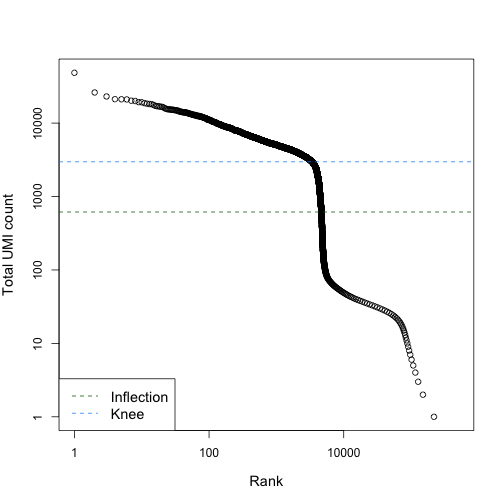
)

set.seed(100)
e.out <- emptyDrops(counts(sce.pbmc))
# See ?emptyDrops for an explanation of why there are NA # values.
summary(e.out$FDR <= 0.001)

##    Mode   FALSE    TRUE    NA's 
## logical    1056    4233  731991

set.seed(100)
limit <- 100
all.out <-
    emptyDrops(counts(sce.pbmc), lower = limit, test.ambient = TRUE)
# Ideally, this histogram should look close to uniform.
# Large peaks near zero indicate that barcodes with total
# counts below 'lower' are not ambient in origin.
hist(all.out$PValue[all.out$Total <= limit &
        all.out$Total > 0],
    xlab = "P-value",
    main = "",
    col = "grey80")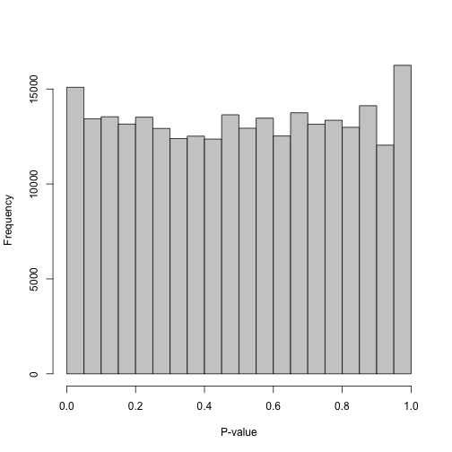

sce.pbmc <- sce.pbmc[, which(e.out$FDR <= 0.001)]
is.mito <- grep("^MT-", rowData(sce.pbmc)$Symbol)
sce.pmbc <- addPerCellQC(sce.pbmc, subsets = list(MT = is.mito))
discard.mito <-
    isOutlier(sce.pmbc$subsets_MT_percent, type = "higher")
plot(
    sce.pmbc$sum,
    sce.pmbc$subsets_MT_percent,
    log = "x",
    xlab = "Total count",
    ylab = "Mitochondrial %"
)
abline(h = attr(discard.mito, "thresholds")["higher"], col = "red")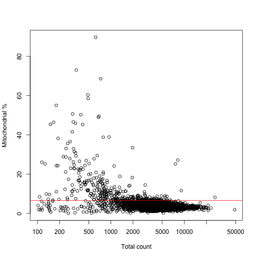

10 / 14

Exercises11 / 14

ExercisesWhy does emptyDrops() return NA values?
11 / 14

Exercises

Why does emptyDrops() return NA values?
Are the p-values the same for e.out and all.out?

11 / 14

Exercises

Why does emptyDrops() return NA values?
Are the p-values the same for e.out and all.out?
What if you subset to the non-NA entries?

11 / 14

Below lower they are considered emptry droplets. Only used for multiple correction testing.
No, due to the NAs.
Yes: identical(e.out$PValue[!is.na(e.out$FDR)], all.out$PValue[!is.na(e.out$FDR)])

# Removing low-quality cells
# Keeping the columns we DON'T want to discard
filtered <- sce.416b[,!discard2]
# Marking low-quality cells
marked <- sce.416b
marked$discard <- discard2

12 / 14

# Removing low-quality cells
# Keeping the columns we DON'T want to discard
filtered <- sce.416b[,!discard2]
# Marking low-quality cells
marked <- sce.416b
marked$discard <- discard2

Which of these objects is larger?

12 / 14

# Removing low-quality cells
# Keeping the columns we DON'T want to discard
filtered <- sce.416b[,!discard2]
# Marking low-quality cells
marked <- sce.416b
marked$discard <- discard2

Which of these objects is larger?
Which one would you prefer to use?

12 / 14

marked is larger than filtered
I would prefer to use the marked one if I have enough memory to do so.

Thanks!

Slides created via the R package xaringan and themed with xaringanthemer.

This course is based on the book Orchestrating Single Cell Analysis with Bioconductor by Aaron Lun, Robert Amezquita, Stephanie Hicks and Raphael Gottardo, plus WEHI's scRNA-seq course by Peter Hickey.

You can find the files for this course at lcolladotor/osca_LIIGH_UNAM_2020.

Instructor: Leonardo Collado-Torres.

Download the materials for this course with usethis::use_course('lcolladotor/osca_LIIGH_UNAM_2020') or view online at lcolladotor.github.io/osca_LIIGH_UNAM_2020.

13 / 14

R session informationoptions(width = 120)
sessioninfo::session_info()

## ─ Session info ───────────────────────────────────────────────────────────────────────────────────────────────────────
##  setting  value                       
##  version  R version 3.6.3 (2020-02-29)
##  os       macOS Catalina 10.15.3      
##  system   x86_64, darwin15.6.0        
##  ui       X11                         
##  language (EN)                        
##  collate  en_US.UTF-8                 
##  ctype    en_US.UTF-8                 
##  tz       America/New_York            
##  date     2020-03-23                  
## 
## ─ Packages ───────────────────────────────────────────────────────────────────────────────────────────────────────────
##  package                * version  date       lib source                                   
##  AnnotationDbi          * 1.48.0   2019-10-29 [1] Bioconductor                             
##  AnnotationFilter       * 1.10.0   2019-10-29 [1] Bioconductor                             
##  AnnotationHub          * 2.18.0   2019-10-29 [1] Bioconductor                             
##  askpass                  1.1      2019-01-13 [1] CRAN (R 3.6.0)                           
##  assertthat               0.2.1    2019-03-21 [1] CRAN (R 3.6.0)                           
##  beeswarm                 0.2.3    2016-04-25 [1] CRAN (R 3.6.0)                           
##  Biobase                * 2.46.0   2019-10-29 [1] Bioconductor                             
##  BiocFileCache          * 1.10.2   2019-11-08 [1] Bioconductor                             
##  BiocGenerics           * 0.32.0   2019-10-29 [1] Bioconductor                             
##  BiocManager              1.30.10  2019-11-16 [1] CRAN (R 3.6.1)                           
##  BiocNeighbors            1.4.2    2020-02-29 [1] Bioconductor                             
##  BiocParallel           * 1.20.1   2019-12-21 [1] Bioconductor                             
##  BiocSingular             1.2.2    2020-02-14 [1] Bioconductor                             
##  BiocVersion              3.10.1   2019-06-06 [1] Bioconductor                             
##  biomaRt                  2.42.0   2019-10-29 [1] Bioconductor                             
##  Biostrings               2.54.0   2019-10-29 [1] Bioconductor                             
##  bit                      1.1-15.2 2020-02-10 [1] CRAN (R 3.6.0)                           
##  bit64                    0.9-7    2017-05-08 [1] CRAN (R 3.6.0)                           
##  bitops                   1.0-6    2013-08-17 [1] CRAN (R 3.6.0)                           
##  blob                     1.2.1    2020-01-20 [1] CRAN (R 3.6.0)                           
##  cli                      2.0.2    2020-02-28 [1] CRAN (R 3.6.0)                           
##  colorout               * 1.2-1    2019-05-07 [1] Github (jalvesaq/colorout@7ea9440)       
##  colorspace               1.4-1    2019-03-18 [1] CRAN (R 3.6.0)                           
##  crayon                   1.3.4    2017-09-16 [1] CRAN (R 3.6.0)                           
##  curl                     4.3      2019-12-02 [1] CRAN (R 3.6.0)                           
##  DBI                      1.1.0    2019-12-15 [1] CRAN (R 3.6.0)                           
##  dbplyr                 * 1.4.2    2019-06-17 [1] CRAN (R 3.6.0)                           
##  DelayedArray           * 0.12.2   2020-01-06 [1] Bioconductor                             
##  DelayedMatrixStats       1.8.0    2019-10-29 [1] Bioconductor                             
##  digest                   0.6.25   2020-02-23 [1] CRAN (R 3.6.0)                           
##  dplyr                    0.8.5    2020-03-07 [1] CRAN (R 3.6.0)                           
##  dqrng                    0.2.1    2019-05-17 [1] CRAN (R 3.6.0)                           
##  DropletUtils           * 1.6.1    2019-10-30 [1] Bioconductor                             
##  edgeR                    3.28.1   2020-02-26 [1] Bioconductor                             
##  ensembldb              * 2.10.2   2019-11-20 [1] Bioconductor                             
##  evaluate                 0.14     2019-05-28 [1] CRAN (R 3.6.0)                           
##  ExperimentHub            1.12.0   2019-10-29 [1] Bioconductor                             
##  fansi                    0.4.1    2020-01-08 [1] CRAN (R 3.6.0)                           
##  fastmap                  1.0.1    2019-10-08 [1] CRAN (R 3.6.0)                           
##  GenomeInfoDb           * 1.22.0   2019-10-29 [1] Bioconductor                             
##  GenomeInfoDbData         1.2.2    2019-10-31 [1] Bioconductor                             
##  GenomicAlignments        1.22.1   2019-11-12 [1] Bioconductor                             
##  GenomicFeatures        * 1.38.2   2020-02-15 [1] Bioconductor                             
##  GenomicRanges          * 1.38.0   2019-10-29 [1] Bioconductor                             
##  ggbeeswarm               0.6.0    2017-08-07 [1] CRAN (R 3.6.0)                           
##  ggplot2                * 3.3.0    2020-03-05 [1] CRAN (R 3.6.0)                           
##  glue                     1.3.2    2020-03-12 [1] CRAN (R 3.6.0)                           
##  gridExtra                2.3      2017-09-09 [1] CRAN (R 3.6.0)                           
##  gtable                   0.3.0    2019-03-25 [1] CRAN (R 3.6.0)                           
##  HDF5Array                1.14.3   2020-02-29 [1] Bioconductor                             
##  hms                      0.5.3    2020-01-08 [1] CRAN (R 3.6.0)                           
##  htmltools                0.4.0    2019-10-04 [1] CRAN (R 3.6.0)                           
##  httpuv                   1.5.2    2019-09-11 [1] CRAN (R 3.6.0)                           
##  httr                     1.4.1    2019-08-05 [1] CRAN (R 3.6.0)                           
##  interactiveDisplayBase   1.24.0   2019-10-29 [1] Bioconductor                             
##  IRanges                * 2.20.2   2020-01-13 [1] Bioconductor                             
##  irlba                    2.3.3    2019-02-05 [1] CRAN (R 3.6.0)                           
##  knitr                    1.28     2020-02-06 [1] CRAN (R 3.6.0)                           
##  later                    1.0.0    2019-10-04 [1] CRAN (R 3.6.0)                           
##  lattice                  0.20-40  2020-02-19 [1] CRAN (R 3.6.0)                           
##  lazyeval                 0.2.2    2019-03-15 [1] CRAN (R 3.6.0)                           
##  lifecycle                0.2.0    2020-03-06 [1] CRAN (R 3.6.0)                           
##  limma                    3.42.2   2020-02-03 [1] Bioconductor                             
##  locfit                   1.5-9.1  2013-04-20 [1] CRAN (R 3.6.0)                           
##  magrittr                 1.5      2014-11-22 [1] CRAN (R 3.6.0)                           
##  Matrix                 * 1.2-18   2019-11-27 [1] CRAN (R 3.6.3)                           
##  matrixStats            * 0.56.0   2020-03-13 [1] CRAN (R 3.6.0)                           
##  memoise                  1.1.0    2017-04-21 [1] CRAN (R 3.6.0)                           
##  mime                     0.9      2020-02-04 [1] CRAN (R 3.6.0)                           
##  munsell                  0.5.0    2018-06-12 [1] CRAN (R 3.6.0)                           
##  openssl                  1.4.1    2019-07-18 [1] CRAN (R 3.6.0)                           
##  pillar                   1.4.3    2019-12-20 [1] CRAN (R 3.6.0)                           
##  pkgconfig                2.0.3    2019-09-22 [1] CRAN (R 3.6.1)                           
##  prettyunits              1.1.1    2020-01-24 [1] CRAN (R 3.6.2)                           
##  progress                 1.2.2    2019-05-16 [1] CRAN (R 3.6.0)                           
##  promises                 1.1.0    2019-10-04 [1] CRAN (R 3.6.0)                           
##  ProtGenerics             1.18.0   2019-10-29 [1] Bioconductor                             
##  purrr                    0.3.3    2019-10-18 [1] CRAN (R 3.6.0)                           
##  R.methodsS3              1.8.0    2020-02-14 [1] CRAN (R 3.6.0)                           
##  R.oo                     1.23.0   2019-11-03 [1] CRAN (R 3.6.0)                           
##  R.utils                  2.9.2    2019-12-08 [1] CRAN (R 3.6.1)                           
##  R6                       2.4.1    2019-11-12 [1] CRAN (R 3.6.1)                           
##  rappdirs                 0.3.1    2016-03-28 [1] CRAN (R 3.6.0)                           
##  Rcpp                     1.0.4    2020-03-17 [1] CRAN (R 3.6.0)                           
##  RCurl                    1.98-1.1 2020-01-19 [1] CRAN (R 3.6.0)                           
##  rhdf5                    2.30.1   2019-11-26 [1] Bioconductor                             
##  Rhdf5lib                 1.8.0    2019-10-29 [1] Bioconductor                             
##  rlang                    0.4.5    2020-03-01 [1] CRAN (R 3.6.0)                           
##  rmarkdown                2.1      2020-01-20 [1] CRAN (R 3.6.0)                           
##  Rsamtools                2.2.3    2020-02-23 [1] Bioconductor                             
##  RSQLite                  2.2.0    2020-01-07 [1] CRAN (R 3.6.0)                           
##  rstudioapi               0.11     2020-02-07 [1] CRAN (R 3.6.0)                           
##  rsvd                     1.0.3    2020-02-17 [1] CRAN (R 3.6.0)                           
##  rtracklayer              1.46.0   2019-10-29 [1] Bioconductor                             
##  S4Vectors              * 0.24.3   2020-01-18 [1] Bioconductor                             
##  scales                   1.1.0    2019-11-18 [1] CRAN (R 3.6.1)                           
##  scater                 * 1.14.6   2019-12-16 [1] Bioconductor                             
##  scRNAseq               * 2.0.2    2019-11-12 [1] Bioconductor                             
##  sessioninfo              1.1.1    2018-11-05 [1] CRAN (R 3.6.0)                           
##  shiny                    1.4.0.2  2020-03-13 [1] CRAN (R 3.6.0)                           
##  SingleCellExperiment   * 1.8.0    2019-10-29 [1] Bioconductor                             
##  stringi                  1.4.6    2020-02-17 [1] CRAN (R 3.6.0)                           
##  stringr                  1.4.0    2019-02-10 [1] CRAN (R 3.6.0)                           
##  SummarizedExperiment   * 1.16.1   2019-12-19 [1] Bioconductor                             
##  tibble                   2.1.3    2019-06-06 [1] CRAN (R 3.6.0)                           
##  tidyselect               1.0.0    2020-01-27 [1] CRAN (R 3.6.0)                           
##  vctrs                    0.2.4    2020-03-10 [1] CRAN (R 3.6.0)                           
##  vipor                    0.4.5    2017-03-22 [1] CRAN (R 3.6.0)                           
##  viridis                  0.5.1    2018-03-29 [1] CRAN (R 3.6.0)                           
##  viridisLite              0.3.0    2018-02-01 [1] CRAN (R 3.6.0)                           
##  withr                    2.1.2    2018-03-15 [1] CRAN (R 3.6.0)                           
##  xaringan                 0.15     2020-03-04 [1] CRAN (R 3.6.3)                           
##  xaringanthemer         * 0.2.0    2020-03-22 [1] Github (gadenbuie/xaringanthemer@460f441)
##  xfun                     0.12     2020-01-13 [1] CRAN (R 3.6.0)                           
##  XML                      3.99-0.3 2020-01-20 [1] CRAN (R 3.6.0)                           
##  xtable                   1.8-4    2019-04-21 [1] CRAN (R 3.6.0)                           
##  XVector                  0.26.0   2019-10-29 [1] Bioconductor                             
##  yaml                     2.2.1    2020-02-01 [1] CRAN (R 3.6.0)                           
##  zlibbioc                 1.32.0   2019-10-29 [1] Bioconductor                             
## 
## [1] /Library/Frameworks/R.framework/Versions/3.6/Resources/library
14 / 14

↑, ←, Pg Up, k	Go to previous slide
↓, →, Pg Dn, Space, j	Go to next slide
Home	Go to first slide
End	Go to last slide
Number + Return	Go to specific slide
b / m / f	Toggle blackout / mirrored / fullscreen mode
c	Clone slideshow
p	Toggle presenter mode
t	Restart the presentation timer
?, h	Toggle this help

Quality Control

Analyzing scRNA-seq data with Bioconductor for LCG-EJ-UNAM March 2020

Leonardo Collado-Torres

2020-03-23

Slides by Peter Hickey

Code and output

Questions

Questions

Questions

QC metrics plots

Questions

Questions

Questions

Questions

Exercises

Exercises

Exercises

Exercises

Thanks!

R session information

Help