5 Modelos estadísticos

• Revisión de regresión lineal https://lcolladotor.github.io/bioc_team_ds/helping-others.html#linear-regression-example
• Con R, usamos mucho la función model.matrix() y la sintáxis de fórmula Y ~ X1 + X2 tal como en el siguiente ejemplo.

## ?model.matrix
mat <- with(trees, model.matrix(log(Volume) ~ log(Height) + log(Girth)))
mat

##    (Intercept) log(Height) log(Girth)
## 1            1    4.248495   2.116256
## 2            1    4.174387   2.151762
## 3            1    4.143135   2.174752
## 4            1    4.276666   2.351375
## 5            1    4.394449   2.370244
## 6            1    4.418841   2.379546
## 7            1    4.189655   2.397895
## 8            1    4.317488   2.397895
## 9            1    4.382027   2.406945
## 10           1    4.317488   2.415914
## 11           1    4.369448   2.424803
## 12           1    4.330733   2.433613
## 13           1    4.330733   2.433613
## 14           1    4.234107   2.459589
## 15           1    4.317488   2.484907
## 16           1    4.304065   2.557227
## 17           1    4.442651   2.557227
## 18           1    4.454347   2.587764
## 19           1    4.262680   2.617396
## 20           1    4.158883   2.624669
## 21           1    4.356709   2.639057
## 22           1    4.382027   2.653242
## 23           1    4.304065   2.674149
## 24           1    4.276666   2.772589
## 25           1    4.343805   2.791165
## 26           1    4.394449   2.850707
## 27           1    4.406719   2.862201
## 28           1    4.382027   2.884801
## 29           1    4.382027   2.890372
## 30           1    4.382027   2.890372
## 31           1    4.465908   3.025291
## attr(,"assign")
## [1] 0 1 2

colnames(mat)

## [1] "(Intercept)" "log(Height)" "log(Girth)"

• ¿Cómo interpretamos los nombres de las columnas de mat?

summary(lm(log(Volume) ~ log(Height) + log(Girth), data = trees))

## 
## Call:
## lm(formula = log(Volume) ~ log(Height) + log(Girth), data = trees)
## 
## Residuals:
##       Min        1Q    Median        3Q       Max 
## -0.168561 -0.048488  0.002431  0.063637  0.129223 
## 
## Coefficients:
##             Estimate Std. Error t value Pr(>|t|)    
## (Intercept) -6.63162    0.79979  -8.292 5.06e-09 ***
## log(Height)  1.11712    0.20444   5.464 7.81e-06 ***
## log(Girth)   1.98265    0.07501  26.432  < 2e-16 ***
## ---
## Signif. codes:  0 '***' 0.001 '**' 0.01 '*' 0.05 '.' 0.1 ' ' 1
## 
## Residual standard error: 0.08139 on 28 degrees of freedom
## Multiple R-squared:  0.9777, Adjusted R-squared:  0.9761 
## F-statistic: 613.2 on 2 and 28 DF,  p-value: < 2.2e-16

5.1 ExploreModelMatrix

• Es un paquete de Bioconductor que nos ayuda a entender los modelos estadísticos que estamos usando gracias a visualizaciones http://www.bioconductor.org/packages/ExploreModelMatrix/ que está descrito en el siguiente artículo
• Revisaremos los ejemplos en http://www.bioconductor.org/packages/release/bioc/vignettes/ExploreModelMatrix/inst/doc/ExploreModelMatrix.html

5.1.1 Ejemplo 1

## Datos de ejemplo
(sampleData <- data.frame(
    genotype = rep(c("A", "B"), each = 4),
    treatment = rep(c("ctrl", "trt"), 4)
))

##   genotype treatment
## 1        A      ctrl
## 2        A       trt
## 3        A      ctrl
## 4        A       trt
## 5        B      ctrl
## 6        B       trt
## 7        B      ctrl
## 8        B       trt

## Creemos las imágenes usando ExploreModelMatrix
vd <- ExploreModelMatrix::VisualizeDesign(
    sampleData = sampleData,
    designFormula = ~ genotype + treatment,
    textSizeFitted = 4
)

## Veamos las imágenes
cowplot::plot_grid(plotlist = vd$plotlist)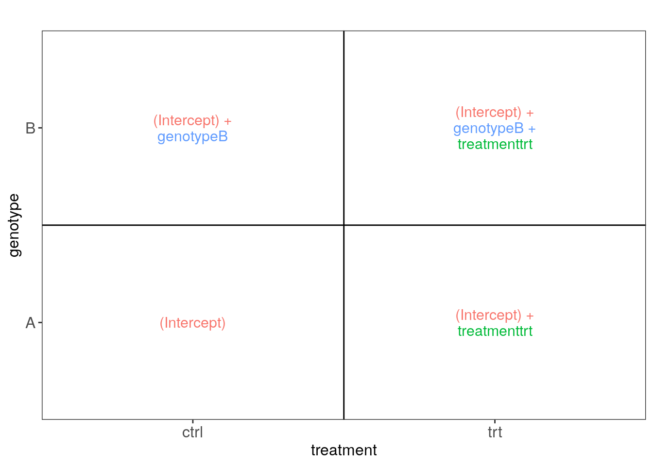

De forma interactiva podemos correr el siguiente código:

## Usaremos shiny otra ves
app <- ExploreModelMatrix(
    sampleData = sampleData,
    designFormula = ~ genotype + treatment
)
if (interactive()) shiny::runApp(app)

5.1.2 Ejemplo 2

http://bioconductor.org/packages/release/bioc/vignettes/ExploreModelMatrix/inst/doc/ExploreModelMatrix.html#example-2

5.1.3 Ejemplo 3

http://bioconductor.org/packages/release/bioc/vignettes/ExploreModelMatrix/inst/doc/ExploreModelMatrix.html#example-3

5.1.4 Ejercicio

• Interpreta ResponseResistant.Treatmentpre del ejercicio 2. Puede ser útil tomar un screenshot (captura de pantalla) y anotarla con líneas de colores. Si haces eso, puedes incluir la imagen en tus notas.
• ¿Por qué es clave el 0 al inicio de la fórmula en el ejercicio 3?

5.1.5 Para aprender más

A guide to creating design matrices for gene expression experiments:

• http://bioconductor.org/packages/release/workflows/vignettes/RNAseq123/inst/doc/designmatrices.html
• https://f1000research.com/articles/9-1444

“Model matrix not full rank”

• http://bioconductor.org/packages/release/bioc/vignettes/DESeq2/inst/doc/DESeq2.html#model-matrix-not-full-rank

5.2 Datos de SRP045638

Vamos a usar datos de https://www.ncbi.nlm.nih.gov/sra/?term=SRP045638 procesados con recount3. Primero hay que descargar los datos con los comandos que vimos ayer.

library("recount3")

options(recount3_url = "https://recount-opendata.s3.amazonaws.com/recount3/release")

human_projects <- available_projects()

## 2023-02-03 00:10:05 caching file sra.recount_project.MD.gz.

## 2023-02-03 00:10:05 caching file gtex.recount_project.MD.gz.

## 2023-02-03 00:10:05 caching file tcga.recount_project.MD.gz.

rse_gene_SRP045638 <- create_rse(
    subset(
        human_projects,
        project == "SRP045638" & project_type == "data_sources"
    )
)

## 2023-02-03 00:10:09 downloading and reading the metadata.

## 2023-02-03 00:10:09 caching file sra.sra.SRP045638.MD.gz.

## adding rname 'https://recount-opendata.s3.amazonaws.com/recount3/release/human/data_sources/sra/metadata/38/SRP045638/sra.sra.SRP045638.MD.gz'

## 2023-02-03 00:10:09 caching file sra.recount_project.SRP045638.MD.gz.

## adding rname 'https://recount-opendata.s3.amazonaws.com/recount3/release/human/data_sources/sra/metadata/38/SRP045638/sra.recount_project.SRP045638.MD.gz'

## 2023-02-03 00:10:10 caching file sra.recount_qc.SRP045638.MD.gz.

## adding rname 'https://recount-opendata.s3.amazonaws.com/recount3/release/human/data_sources/sra/metadata/38/SRP045638/sra.recount_qc.SRP045638.MD.gz'

## 2023-02-03 00:10:10 caching file sra.recount_seq_qc.SRP045638.MD.gz.

## adding rname 'https://recount-opendata.s3.amazonaws.com/recount3/release/human/data_sources/sra/metadata/38/SRP045638/sra.recount_seq_qc.SRP045638.MD.gz'

## 2023-02-03 00:10:11 caching file sra.recount_pred.SRP045638.MD.gz.

## adding rname 'https://recount-opendata.s3.amazonaws.com/recount3/release/human/data_sources/sra/metadata/38/SRP045638/sra.recount_pred.SRP045638.MD.gz'

## 2023-02-03 00:10:11 downloading and reading the feature information.

## 2023-02-03 00:10:11 caching file human.gene_sums.G026.gtf.gz.

## 2023-02-03 00:10:12 downloading and reading the counts: 66 samples across 63856 features.

## 2023-02-03 00:10:12 caching file sra.gene_sums.SRP045638.G026.gz.

## adding rname 'https://recount-opendata.s3.amazonaws.com/recount3/release/human/data_sources/sra/gene_sums/38/SRP045638/sra.gene_sums.SRP045638.G026.gz'

## 2023-02-03 00:10:12 construcing the RangedSummarizedExperiment (rse) object.

assay(rse_gene_SRP045638, "counts") <- compute_read_counts(rse_gene_SRP045638)

Una vez descargados y con los números de lecturas podemos usar expand_sra_attributes(). Sin embargo, tenemos un problema con estos datos.

rse_gene_SRP045638$sra.sample_attributes[1:3]

## [1] "age;;67.78|biomaterial_provider;;LIBD|BioSampleModel;;Human|dev_stage;;Fetal|disease;;Control|Fraction;;total|isolate;;DLPFC|race;;AA|RIN;;8.3|sex;;female|tissue;;DLPFC"
## [2] "age;;40.42|biomaterial_provider;;LIBD|BioSampleModel;;Human|disease;;Control|Fraction;;total|isolate;;DLPFC|race;;AA|RIN;;8.4|sex;;male|tissue;;DLPFC"                   
## [3] "age;;41.58|biomaterial_provider;;LIBD|BioSampleModel;;Human|disease;;control|Fraction;;total|isolate;;R2869|race;;AA|RIN;;8.7|sex;;male|tissue;;DLPFC"

Vamos a intentar resolverlo eliminando información que está presente solo en ciertas muestras.

rse_gene_SRP045638$sra.sample_attributes <- gsub("dev_stage;;Fetal\\|", "", rse_gene_SRP045638$sra.sample_attributes)
rse_gene_SRP045638$sra.sample_attributes[1:3]

## [1] "age;;67.78|biomaterial_provider;;LIBD|BioSampleModel;;Human|disease;;Control|Fraction;;total|isolate;;DLPFC|race;;AA|RIN;;8.3|sex;;female|tissue;;DLPFC"
## [2] "age;;40.42|biomaterial_provider;;LIBD|BioSampleModel;;Human|disease;;Control|Fraction;;total|isolate;;DLPFC|race;;AA|RIN;;8.4|sex;;male|tissue;;DLPFC"  
## [3] "age;;41.58|biomaterial_provider;;LIBD|BioSampleModel;;Human|disease;;control|Fraction;;total|isolate;;R2869|race;;AA|RIN;;8.7|sex;;male|tissue;;DLPFC"

Ahora si podemos continuar con el mismo código de ayer.

rse_gene_SRP045638 <- expand_sra_attributes(rse_gene_SRP045638)

colData(rse_gene_SRP045638)[
    ,
    grepl("^sra_attribute", colnames(colData(rse_gene_SRP045638)))
]

## DataFrame with 66 rows and 10 columns
##            sra_attribute.age sra_attribute.biomaterial_provider sra_attribute.BioSampleModel sra_attribute.disease
##                  <character>                        <character>                  <character>           <character>
## SRR2071341             67.78                               LIBD                        Human               Control
## SRR2071345             40.42                               LIBD                        Human               Control
## SRR2071346             41.58                               LIBD                        Human               control
## SRR2071347             44.17                               LIBD                        Human               control
## SRR2071348           -0.3836                               LIBD                        Human               control
## ...                      ...                                ...                          ...                   ...
## SRR2071366             66.72                               LIBD                        Human               control
## SRR2071372             43.88                               LIBD                        Human               control
## SRR2071373             15.17                               LIBD                        Human               control
## SRR2071374             70.95                               LIBD                        Human               control
## SRR2071375              4.14                               LIBD                        Human               control
##            sra_attribute.Fraction sra_attribute.isolate sra_attribute.race sra_attribute.RIN sra_attribute.sex
##                       <character>           <character>        <character>       <character>       <character>
## SRR2071341                  total                 DLPFC                 AA               8.3            female
## SRR2071345                  total                 DLPFC                 AA               8.4              male
## SRR2071346                  total                 R2869                 AA               8.7              male
## SRR2071347                  total                 R3098                 AA               5.3            female
## SRR2071348                  total                 R3452                 AA               9.6            female
## ...                           ...                   ...                ...               ...               ...
## SRR2071366                  total                 R3763               CAUC                 7            female
## SRR2071372                  total                 R4166                 AA               8.7              male
## SRR2071373                  total                 R4196               CAUC               7.9            female
## SRR2071374                  total                 R4338                 AS               8.3              male
## SRR2071375                  total                 R4699               CAUC               8.7              male
##            sra_attribute.tissue
##                     <character>
## SRR2071341                DLPFC
## SRR2071345                DLPFC
## SRR2071346                DLPFC
## SRR2071347                DLPFC
## SRR2071348                DLPFC
## ...                         ...
## SRR2071366                DLPFC
## SRR2071372                DLPFC
## SRR2071373                DLPFC
## SRR2071374                DLPFC
## SRR2071375                DLPFC

Como ahora si vamos a usar esta información para un modelo estadístico, será importante que tengamos en el formato correcto de R a la información que vamos a usar.

## Pasar de character a numeric o factor
rse_gene_SRP045638$sra_attribute.age <- as.numeric(rse_gene_SRP045638$sra_attribute.age)
rse_gene_SRP045638$sra_attribute.disease <- factor(tolower(rse_gene_SRP045638$sra_attribute.disease))
rse_gene_SRP045638$sra_attribute.RIN <- as.numeric(rse_gene_SRP045638$sra_attribute.RIN)
rse_gene_SRP045638$sra_attribute.sex <- factor(rse_gene_SRP045638$sra_attribute.sex)

## Resumen de las variables de interés
summary(as.data.frame(colData(rse_gene_SRP045638)[
    ,
    grepl("^sra_attribute.[age|disease|RIN|sex]", colnames(colData(rse_gene_SRP045638)))
]))

##  sra_attribute.age sra_attribute.disease sra_attribute.isolate sra_attribute.RIN sra_attribute.sex
##  Min.   :-0.4986   control:66            Length:66             Min.   :5.30      female:22        
##  1st Qu.: 0.3424                         Class :character      1st Qu.:8.00      male  :44        
##  Median :14.9000                         Mode  :character      Median :8.30                       
##  Mean   :22.6286                                               Mean   :8.15                       
##  3rd Qu.:41.2900                                               3rd Qu.:8.70                       
##  Max.   :73.9100                                               Max.   :9.60

Ahora crearemos un par de variables para que las podamos usar en nuestro análisis.

## Encontraremos diferencias entre muestra prenatalas vs postnatales
rse_gene_SRP045638$prenatal <- factor(ifelse(rse_gene_SRP045638$sra_attribute.age < 0, "prenatal", "postnatal"))
table(rse_gene_SRP045638$prenatal)

## 
## postnatal  prenatal 
##        56        10

## http://rna.recount.bio/docs/quality-check-fields.html
rse_gene_SRP045638$assigned_gene_prop <- rse_gene_SRP045638$recount_qc.gene_fc_count_all.assigned / rse_gene_SRP045638$recount_qc.gene_fc_count_all.total
summary(rse_gene_SRP045638$assigned_gene_prop)

##    Min. 1st Qu.  Median    Mean 3rd Qu.    Max. 
##  0.1942  0.7004  0.7591  0.7170  0.7991  0.8493

with(colData(rse_gene_SRP045638), plot(assigned_gene_prop, sra_attribute.RIN))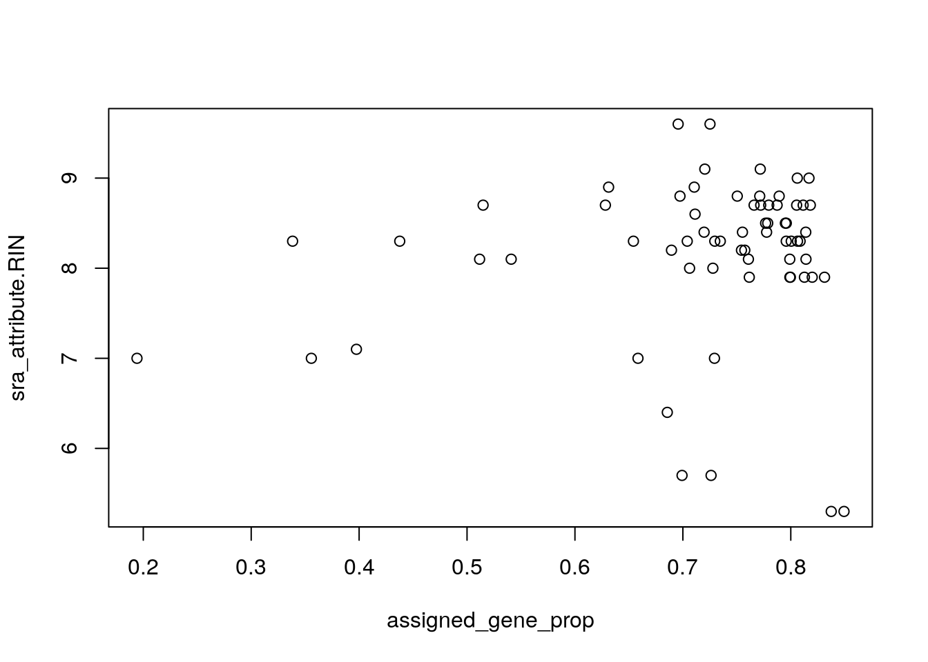

## Hm... veamos si hay una diferencia entre los grupos
with(colData(rse_gene_SRP045638), tapply(assigned_gene_prop, prenatal, summary))

## $postnatal
##    Min. 1st Qu.  Median    Mean 3rd Qu.    Max. 
##  0.1942  0.7072  0.7719  0.7179  0.8017  0.8493 
## 
## $prenatal
##    Min. 1st Qu.  Median    Mean 3rd Qu.    Max. 
##  0.6856  0.7004  0.7088  0.7116  0.7259  0.7347

A continuación podemos eliminar algunas muestras que consideremos de baja calidad y genes con niveles de expresión muy bajos.

## Guardemos nuestro objeto entero por si luego cambiamos de opinión
rse_gene_SRP045638_unfiltered <- rse_gene_SRP045638

## Eliminemos a muestras malas
hist(rse_gene_SRP045638$assigned_gene_prop)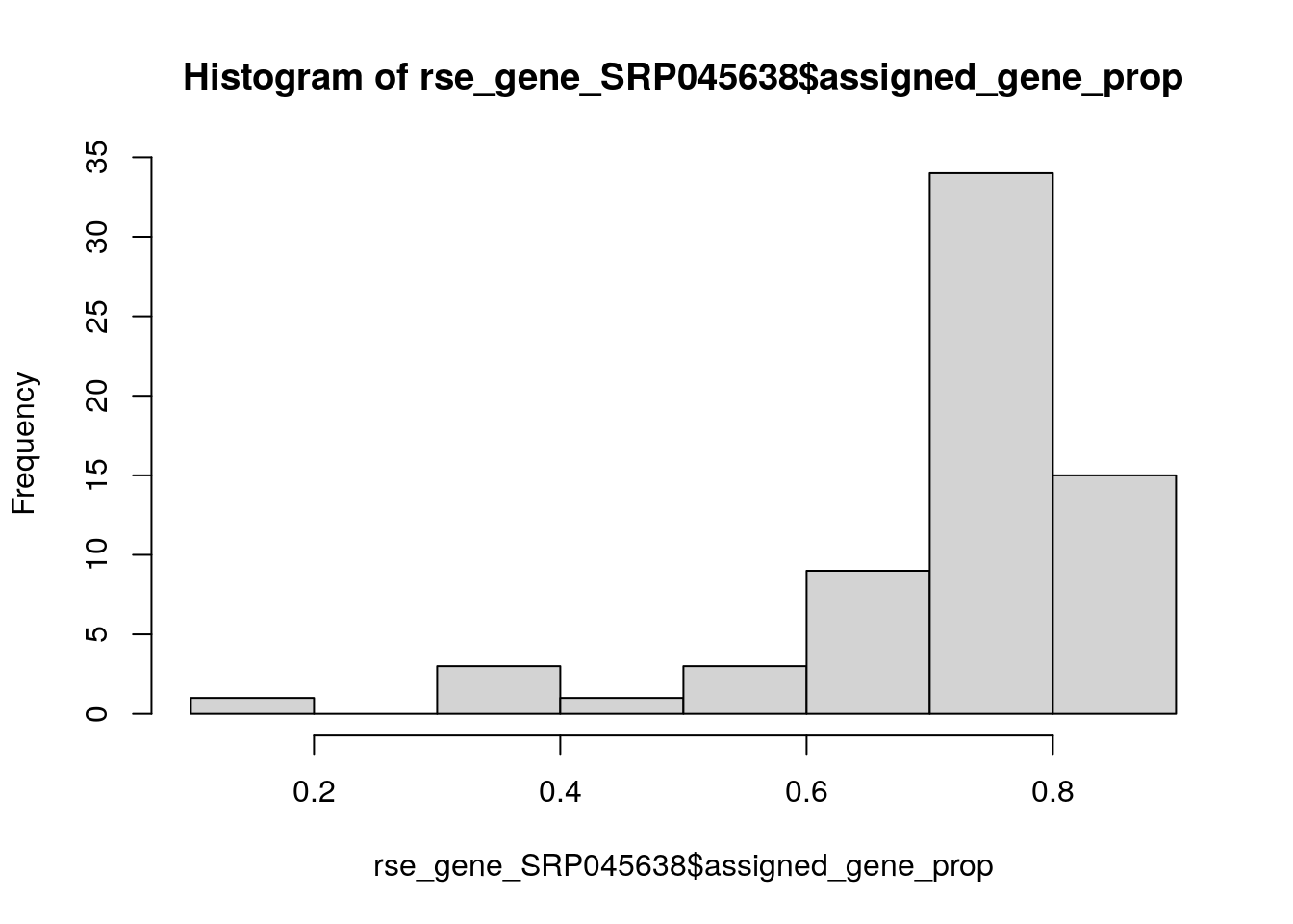

table(rse_gene_SRP045638$assigned_gene_prop < 0.3)

## 
## FALSE  TRUE 
##    65     1

rse_gene_SRP045638 <- rse_gene_SRP045638[, rse_gene_SRP045638$assigned_gene_prop > 0.3]

## Calculemos los niveles medios de expresión de los genes en nuestras
## muestras.
## Ojo: en un análisis real probablemente haríamos esto con los RPKMs o CPMs
## en vez de las cuentas.
## En realidad usariamos:
# edgeR::filterByExpr() https://bioconductor.org/packages/edgeR/ https://rdrr.io/bioc/edgeR/man/filterByExpr.html
# genefilter::genefilter() https://bioconductor.org/packages/genefilter/ https://rdrr.io/bioc/genefilter/man/genefilter.html
# jaffelab::expression_cutoff() http://research.libd.org/jaffelab/reference/expression_cutoff.html
#
gene_means <- rowMeans(assay(rse_gene_SRP045638, "counts"))
summary(gene_means)

##      Min.   1st Qu.    Median      Mean   3rd Qu.      Max. 
##       0.0       0.1       2.5     815.2     170.2 1362047.9

## Eliminamos genes
rse_gene_SRP045638 <- rse_gene_SRP045638[gene_means > 0.1, ]

## Dimensiones finales
dim(rse_gene_SRP045638)

## [1] 46929    65

## Porcentaje de genes que retuvimos
round(nrow(rse_gene_SRP045638) / nrow(rse_gene_SRP045638_unfiltered) * 100, 2)

## [1] 73.49

Ahora ya estamos listos para continuar con el análisis de expresión diferencial, bueno, casi.

5.3 Normalización de datos

• Lean A hypothetical scenario en uno de los artículos sobre edgeR https://genomebiology.biomedcentral.com/articles/10.1186/gb-2010-11-3-r25#Sec2 para entender un poco sobre el concepto de composition bias.
• Sigue siendo relevante con datos de scRNA-seq como pueden ver en http://bioconductor.org/books/3.16/OSCA.multisample/multi-sample-comparisons.html#performing-the-de-analysis. Ahí descubren una serie de pasos para usar métodos desarrollados para bulk RNA-seq y como se pueden usar en scRNA-seq.

library("edgeR") # BiocManager::install("edgeR", update = FALSE)
dge <- DGEList(
    counts = assay(rse_gene_SRP045638, "counts"),
    genes = rowData(rse_gene_SRP045638)
)
dge <- calcNormFactors(dge)

5.4 Expresión diferencial

Primero que nada, definamos nuestro modelo estadístico. Típicamente, exploraríamos más los datos para revisar que no haya otros problemas con las muestras y para explorar la relación entre nuestras variables.

library("ggplot2")
ggplot(as.data.frame(colData(rse_gene_SRP045638)), aes(y = assigned_gene_prop, x = prenatal)) +
    geom_boxplot() +
    theme_bw(base_size = 20) +
    ylab("Assigned Gene Prop") +
    xlab("Age Group")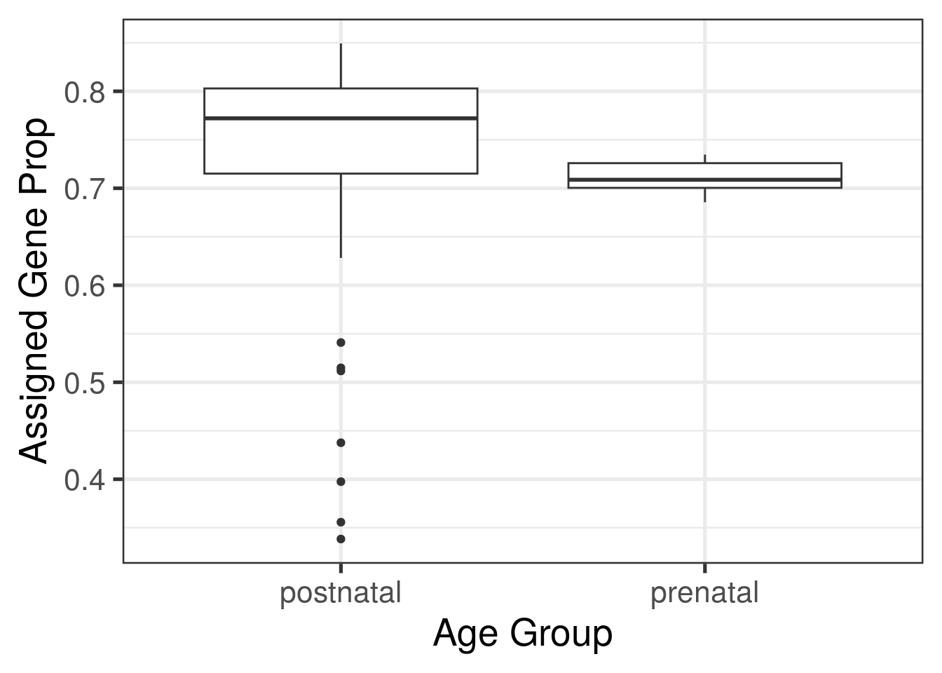

Por ejemplo, usando el paquete de variancePartition y scater entre otros tal como exploramos en el siguiente video del club de R de LIBD (notes in English)/

Por ahora continuaremos con el siguiente modelo estadístico.

mod <- model.matrix(~ prenatal + sra_attribute.RIN + sra_attribute.sex + assigned_gene_prop,
    data = colData(rse_gene_SRP045638)
)
colnames(mod)

## [1] "(Intercept)"           "prenatalprenatal"      "sra_attribute.RIN"     "sra_attribute.sexmale"
## [5] "assigned_gene_prop"

Ya teniendo el modelo estadístico, podemos usar limma para realizar el análisis de expresión diferencial como tal.

library("limma")
vGene <- voom(dge, mod, plot = TRUE)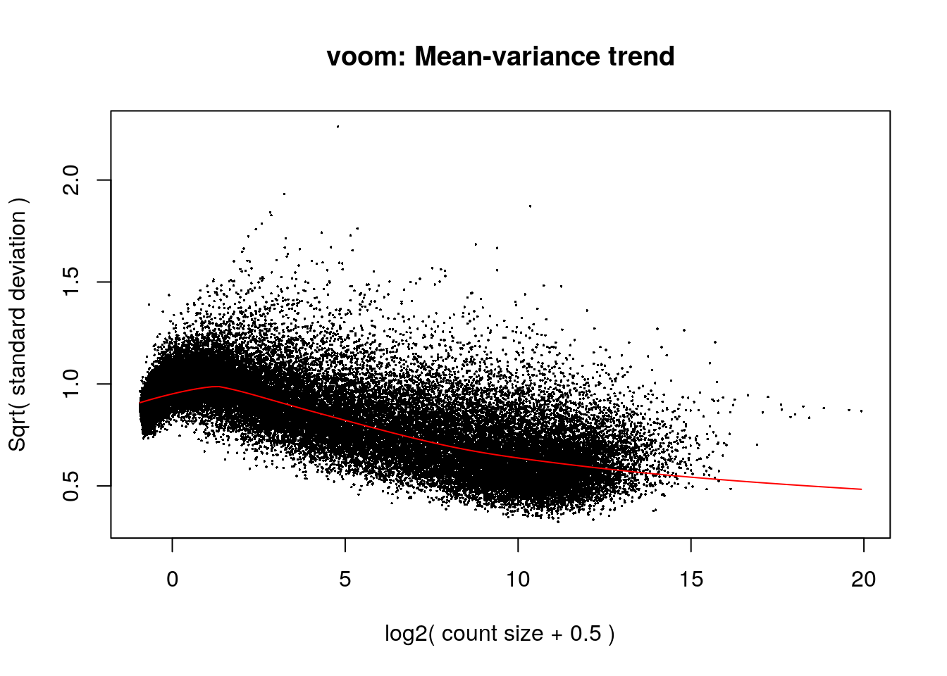

eb_results <- eBayes(lmFit(vGene))

de_results <- topTable(
    eb_results,
    coef = 2,
    number = nrow(rse_gene_SRP045638),
    sort.by = "none"
)
dim(de_results)

## [1] 46929    16

head(de_results)

##                    source type bp_length phase           gene_id                          gene_type   gene_name level
## ENSG00000223972.5  HAVANA gene      1735    NA ENSG00000223972.5 transcribed_unprocessed_pseudogene     DDX11L1     2
## ENSG00000278267.1 ENSEMBL gene        68    NA ENSG00000278267.1                              miRNA   MIR6859-1     3
## ENSG00000227232.5  HAVANA gene      1351    NA ENSG00000227232.5             unprocessed_pseudogene      WASH7P     2
## ENSG00000284332.1 ENSEMBL gene       138    NA ENSG00000284332.1                              miRNA   MIR1302-2     3
## ENSG00000243485.5  HAVANA gene      1021    NA ENSG00000243485.5                            lincRNA MIR1302-2HG     2
## ENSG00000237613.2  HAVANA gene      1219    NA ENSG00000237613.2                            lincRNA     FAM138A     2
##                            havana_gene        tag      logFC    AveExpr         t      P.Value    adj.P.Val          B
## ENSG00000223972.5 OTTHUMG00000000961.2       <NA> -0.4522185 -3.4441644 -1.637034 1.064080e-01 1.348462e-01 -5.5544843
## ENSG00000278267.1                 <NA>       <NA>  1.1158860 -1.3116448  6.123756 5.743771e-08 2.105690e-07  7.7639118
## ENSG00000227232.5 OTTHUMG00000000958.1       <NA>  0.6860298  3.6411313  5.644804 3.816951e-07 1.247133e-06  5.5007844
## ENSG00000284332.1                 <NA>       <NA>  0.4559904 -5.7311063  1.438080 1.551609e-01 1.903075e-01 -5.7956155
## ENSG00000243485.5 OTTHUMG00000000959.2 ncRNA_host  0.9640252 -0.6646248  5.072618 3.445542e-06 9.728406e-06  3.7022021
## ENSG00000237613.2 OTTHUMG00000000960.1       <NA> -1.5460829 -5.3019159 -4.190983 8.476784e-05 1.828325e-04  0.9292571

## Genes diferencialmente expresados entre pre y post natal con FDR < 5%
table(de_results$adj.P.Val < 0.05)

## 
## FALSE  TRUE 
## 12851 34078

## Visualicemos los resultados estadísticos
plotMA(eb_results, coef = 2)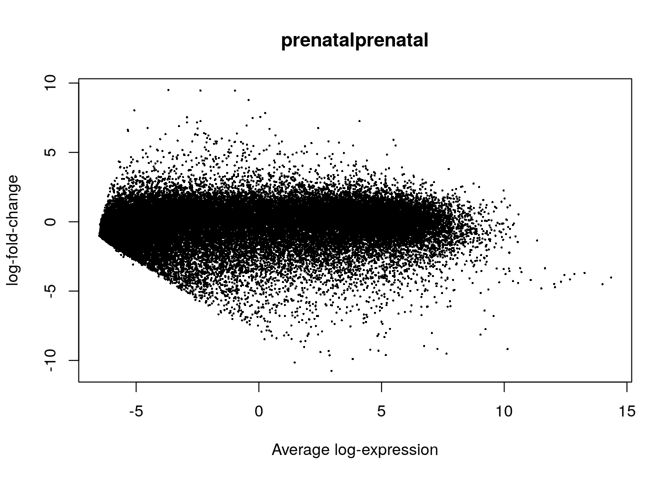

volcanoplot(eb_results, coef = 2, highlight = 3, names = de_results$gene_name)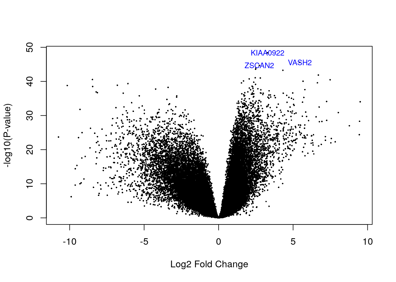

de_results[de_results$gene_name %in% c("ZSCAN2", "VASH2", "KIAA0922"), ]

##                    source type bp_length phase            gene_id      gene_type gene_name level          havana_gene
## ENSG00000143494.15 HAVANA gene      9086    NA ENSG00000143494.15 protein_coding     VASH2     2 OTTHUMG00000036925.5
## ENSG00000176371.13 HAVANA gene      4878    NA ENSG00000176371.13 protein_coding    ZSCAN2     1 OTTHUMG00000074027.5
## ENSG00000121210.15 HAVANA gene      6393    NA ENSG00000121210.15 protein_coding  KIAA0922     2 OTTHUMG00000153244.5
##                     tag    logFC  AveExpr        t      P.Value    adj.P.Val         B
## ENSG00000143494.15 <NA> 5.444271 1.876990 37.85216 2.561452e-46 6.010319e-42  95.10126
## ENSG00000176371.13 <NA> 2.735639 2.751109 36.59344 2.137022e-45 3.342943e-41  92.99949
## ENSG00000121210.15 <NA> 3.283050 2.945269 41.89725 4.235912e-49 1.987871e-44 101.31124

• https://www.genecards.org/cgi-bin/carddisp.pl?gene=ZSCAN2
• https://www.genecards.org/cgi-bin/carddisp.pl?gene=VASH2
• https://www.genecards.org/cgi-bin/carddisp.pl?gene=KIAA0922

5.5 Visualizando genes DE

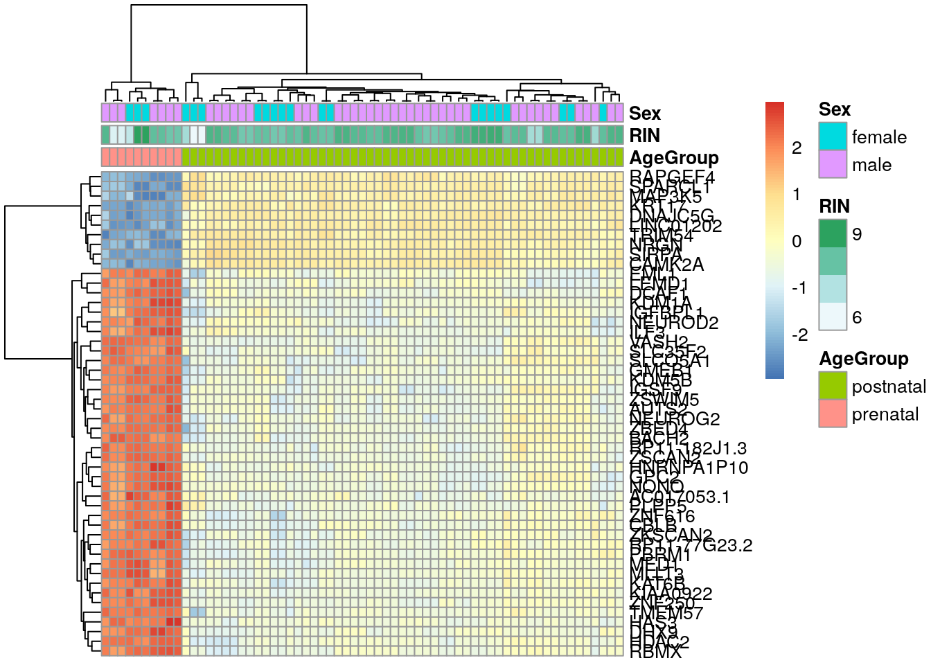
De vGene$E podemos extraer los datos normalizados por limma-voom. Revisemos los top 50 genes diferencialmente expresados.

## Extraer valores de los genes de interés
exprs_heatmap <- vGene$E[rank(de_results$adj.P.Val) <= 50, ]

## Creemos una tabla con información de las muestras
## y con nombres de columnas más amigables
df <- as.data.frame(colData(rse_gene_SRP045638)[, c("prenatal", "sra_attribute.RIN", "sra_attribute.sex")])
colnames(df) <- c("AgeGroup", "RIN", "Sex")

## Hagamos un heatmap
library("pheatmap")
pheatmap(
    exprs_heatmap,
    cluster_rows = TRUE,
    cluster_cols = TRUE,
    show_rownames = FALSE,
    show_colnames = FALSE,
    annotation_col = df
)

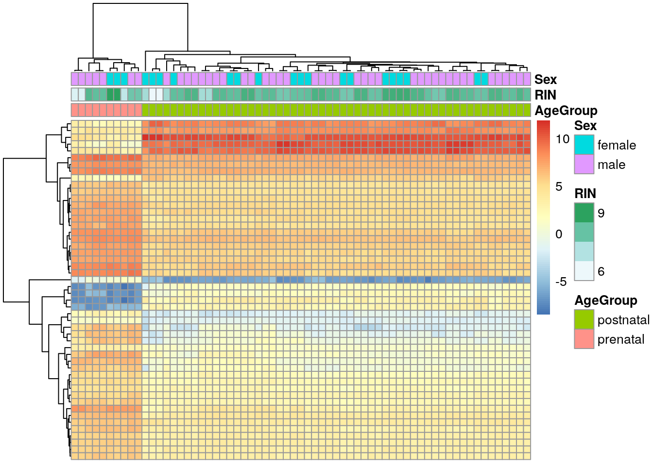
Los resultados que tenemos no son tan sorprendentes porque hay una diferencia enorme en los perfiles de expresión en el DLPFC entre muestra pre y post-natales. Eso lo podemos ver con MDS (multidimensional scaling) tal como describen en este workflow.

## Para colores
library("RColorBrewer")

## Conviertiendo los grupos de edad a colores
col.group <- df$AgeGroup
levels(col.group) <- brewer.pal(nlevels(col.group), "Set1")

## Warning in brewer.pal(nlevels(col.group), "Set1"): minimal value for n is 3, returning requested palette with 3 different levels

col.group <- as.character(col.group)

## MDS por grupos de edad
plotMDS(vGene$E, labels = df$AgeGroup, col = col.group)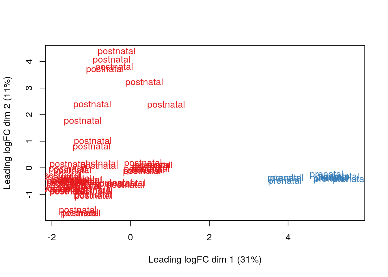

## Conviertiendo los valores de Sex a colores
col.sex <- df$Sex
levels(col.sex) <- brewer.pal(nlevels(col.sex), "Dark2")

## Warning in brewer.pal(nlevels(col.sex), "Dark2"): minimal value for n is 3, returning requested palette with 3 different levels

col.sex <- as.character(col.sex)

## MDS por sexo
plotMDS(vGene$E, labels = df$Sex, col = col.sex)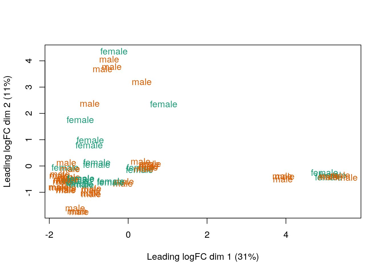

5.6 Ejercicio

Agreguen los nombres de los genes a nuestro pheatmap.

Pistas:

• Revisen la información de rowRanges(rse_gene_SRP045638) o de_results.
• Exploren que hace la función match().

5.7 Comunidad

Algunxs de lxs autores de ExploreModelMatrix:

• https://twitter.com/CSoneson
• https://twitter.com/FedeBioinfo
• https://twitter.com/mikelove

Algunxs de lxs autores de edgeR y limma:

• https://twitter.com/mritchieau
• https://twitter.com/davisjmcc
• https://twitter.com/markrobinsonca
• https://twitter.com/AliciaOshlack

If you've ever been dazed by design matrices or confused by contrasts when performing gene expression analysis in limma, the new article by Charity Law is for you https://t.co/ZSMOA20tdm #bioconductor #rstats (1/2)

— Matt Ritchie (@mritchieau) December 15, 2020

5.8 Ejercicio: respuesta

## Tenemos que usar gene_id y gene_name
rowRanges(rse_gene_SRP045638)

## GRanges object with 46929 ranges and 10 metadata columns:
##                     seqnames            ranges strand |   source     type bp_length     phase           gene_id
##                        <Rle>         <IRanges>  <Rle> | <factor> <factor> <numeric> <integer>       <character>
##   ENSG00000223972.5     chr1       11869-14409      + |  HAVANA      gene      1735      <NA> ENSG00000223972.5
##   ENSG00000278267.1     chr1       17369-17436      - |  ENSEMBL     gene        68      <NA> ENSG00000278267.1
##   ENSG00000227232.5     chr1       14404-29570      - |  HAVANA      gene      1351      <NA> ENSG00000227232.5
##   ENSG00000284332.1     chr1       30366-30503      + |  ENSEMBL     gene       138      <NA> ENSG00000284332.1
##   ENSG00000243485.5     chr1       29554-31109      + |  HAVANA      gene      1021      <NA> ENSG00000243485.5
##                 ...      ...               ...    ... .      ...      ...       ...       ...               ...
##   ENSG00000229238.3     chrY 26277923-26354418      - |   HAVANA     gene      1671      <NA> ENSG00000229238.3
##   ENSG00000224240.1     chrY 26549425-26549743      + |   HAVANA     gene       319      <NA> ENSG00000224240.1
##   ENSG00000215506.5     chrY 26508213-26579690      + |   HAVANA     gene      1605      <NA> ENSG00000215506.5
##   ENSG00000231514.1     chrY 26626520-26627159      - |   HAVANA     gene       640      <NA> ENSG00000231514.1
##   ENSG00000237917.1     chrY 26594851-26634652      - |   HAVANA     gene      2337      <NA> ENSG00000237917.1
##                                  gene_type   gene_name       level          havana_gene               tag
##                                <character> <character> <character>          <character>       <character>
##   ENSG00000223972.5 transcribed_unproces..     DDX11L1           2 OTTHUMG00000000961.2              <NA>
##   ENSG00000278267.1                  miRNA   MIR6859-1           3                 <NA>              <NA>
##   ENSG00000227232.5 unprocessed_pseudogene      WASH7P           2 OTTHUMG00000000958.1              <NA>
##   ENSG00000284332.1                  miRNA   MIR1302-2           3                 <NA>              <NA>
##   ENSG00000243485.5                lincRNA MIR1302-2HG           2 OTTHUMG00000000959.2        ncRNA_host
##                 ...                    ...         ...         ...                  ...               ...
##   ENSG00000229238.3 unprocessed_pseudogene  PPP1R12BP1           2 OTTHUMG00000036764.2              <NA>
##   ENSG00000224240.1   processed_pseudogene     CYCSP49           1 OTTHUMG00000036760.1 overlapping_locus
##   ENSG00000215506.5 unprocessed_pseudogene     TPTE2P4           1 OTTHUMG00000036765.1 overlapping_locus
##   ENSG00000231514.1   processed_pseudogene     FAM58CP           1 OTTHUMG00000036813.1 overlapping_locus
##   ENSG00000237917.1 unprocessed_pseudogene     PARP4P1           1 OTTHUMG00000036812.1 overlapping_locus
##   -------
##   seqinfo: 374 sequences from an unspecified genome; no seqlengths

## Alternativamente, podriamos haber usado de_results
head(de_results, n = 3)

##                    source type bp_length phase           gene_id                          gene_type gene_name level
## ENSG00000223972.5  HAVANA gene      1735    NA ENSG00000223972.5 transcribed_unprocessed_pseudogene   DDX11L1     2
## ENSG00000278267.1 ENSEMBL gene        68    NA ENSG00000278267.1                              miRNA MIR6859-1     3
## ENSG00000227232.5  HAVANA gene      1351    NA ENSG00000227232.5             unprocessed_pseudogene    WASH7P     2
##                            havana_gene  tag      logFC   AveExpr         t      P.Value    adj.P.Val         B
## ENSG00000223972.5 OTTHUMG00000000961.2 <NA> -0.4522185 -3.444164 -1.637034 1.064080e-01 1.348462e-01 -5.554484
## ENSG00000278267.1                 <NA> <NA>  1.1158860 -1.311645  6.123756 5.743771e-08 2.105690e-07  7.763912
## ENSG00000227232.5 OTTHUMG00000000958.1 <NA>  0.6860298  3.641131  5.644804 3.816951e-07 1.247133e-06  5.500784

## Es la misma información
identical(rowRanges(rse_gene_SRP045638)$gene_id, de_results$gene_id)

## [1] TRUE

identical(rowRanges(rse_gene_SRP045638)$gene_name, de_results$gene_name)

## [1] TRUE

## Guardemos los IDs de nuestros 50 genes
nombres_originales <- rownames(exprs_heatmap)

## Con match() podemos encontrar cual es cual
rownames(exprs_heatmap) <- rowRanges(rse_gene_SRP045638)$gene_name[
    match(rownames(exprs_heatmap), rowRanges(rse_gene_SRP045638)$gene_id)
]

## Vean que tambien podriamos haber usado rank()
identical(
    which(rank(de_results$adj.P.Val) <= 50),
    match(nombres_originales, rowRanges(rse_gene_SRP045638)$gene_id)
)

## [1] TRUE

## Esta es otra solución
identical(
    de_results$gene_name[rank(de_results$adj.P.Val) <= 50],
    rownames(exprs_heatmap)
)

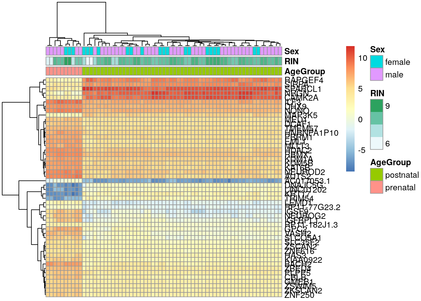
## [1] TRUE

## Por último podemos cambiar el valor de show_rownames de FALSE a TRUE
pheatmap(
    exprs_heatmap,
    cluster_rows = TRUE,
    cluster_cols = TRUE,
    show_rownames = TRUE,
    show_colnames = FALSE,
    annotation_col = df
)

## Guardar la imagen en un PDF largo para poder ver los nombres de los genes
pdf("pheatmap_con_nombres.pdf", height = 14, useDingbats = FALSE)
pheatmap(
    exprs_heatmap,
    cluster_rows = TRUE,
    cluster_cols = TRUE,
    show_rownames = TRUE,
    show_colnames = FALSE,
    annotation_col = df
)
dev.off()

## pdf 
##   3

5.9 Sobre centering y scaling en heatmaps

## Versión con centering y scaling en los renglones (los genes)
pheatmap::pheatmap(
    exprs_heatmap,
    cluster_rows = TRUE,
    cluster_cols = TRUE,
    show_rownames = TRUE,
    show_colnames = FALSE,
    annotation_col = df,
    scale = "row"
)

También podemos hacer una versión con ComplexHeatmap https://bioconductor.org/packages/ComplexHeatmap/.

## Misma versión pero ahora con ComplexHeatmap en vez del paquete pheatmap
ComplexHeatmap::pheatmap(
    exprs_heatmap,
    cluster_rows = TRUE,
    cluster_cols = TRUE,
    show_rownames = TRUE,
    show_colnames = FALSE,
    annotation_col = df,
    scale = "row"
)

5.10 Específicaciones del proyecto

• Con datos de algún estudio disponible vía recount3, hagan un análisis de expresión diferencial.
• Incluyan al menos 3 gráficas en su reporte.
• Incluyan al menos un párrafo de interpretación biológica de los resultados.
• Su reporte debe ser público y estar listado en la página del curso.

Suena fácil, pero cada estudio tiene sus complejidades.

Hay muchos paquetes que no vimos que les pueden llamar la atención, tal como ideal. En http://research.libd.org/SPEAQeasy-example/bootcamp_intro pueden encontrar varias gráficas que tal vez les quieran reproducir. En fin, ¡esto solo es el inicio!

🎉🎉🎉Our new MS is finally out! Given the timing, Santa had an early round with us 🎅
💡https://t.co/a0dHFGWN7V, "ideal: an R/Bioconductor package for interactive differential expression analysis".

I promise a proper #rstats hexsticker will follow, for now enjoy the package 😉

— Federico Marini (@FedeBioinfo) December 10, 2020

© 2011-2020. All thoughts and opinions here are my own. The icon was designed by Mauricio Guzmán and is inspired by Huichol culture; it represents my community building interests.

This work is licensed under CC BY NC SA 4.0

Published with Bookdown