derfinder users guide
Leonardo Collado-Torres
Lieber Institute for Brain Development, Johns Hopkins Medical CampusCenter for Computational Biology, Johns Hopkins Universitylcolladotor@gmail.com
31 March 2026
Source:vignettes/derfinder-users-guide.Rmd
derfinder-users-guide.RmdAsking for help
Please read the basics
of using derfinder in the quick start guide. Thank
you.
derfinder users guide
If you haven’t already, please read the quick start to using derfinder vignette. It explains the basics of using derfinder, how to ask for help, and showcases an example analysis.
The derfinder users guide goes into more depth about what you can do with derfinder. It covers the two implementations of the DER Finder approach (Frazee, Sabunciyan, Hansen, Irizarry, and Leek, 2014). That is, the (A) expressed regions-level and (B) single base-level F-statistics implementations. The vignette also includes advanced material for fine tuning some options, working with non-human data, and example scripts for a high-performance computing cluster.
Expressed regions-level
The expressed regions-level implementation is based on summarizing the coverage information for all your samples and applying a cutoff to that summary. For example, by calculating the mean coverage at every base and then checking if it’s greater than some cutoff value of interest. Contiguous bases passing the cutoff become a candidate Expressed Region (ER). We can then construct a matrix summarizing the base-level coverage for each sample for the set of ERs. This matrix can then be using with packages developed for feature counting (limma, DESeq2, edgeR, etc) to determine which ERs have differential expression signal. That is, to identify the Differentially Expressed Regions (DERs).
regionMatrix()
Commonly, users have aligned their raw RNA-seq data and saved the alignments in BAM files. Some might have chosen to compress this information into BigWig files. BigWig files are much faster to load than BAM files and are the type of file we prefer to work with. However, we can still identify the expressed regions from BAM files.
The function regionMatrix() will require you to load the
data (either from BAM or BigWig files) and store it all in memory. It
will then calculate the mean coverage across all samples, apply the
cutoff you chose, and determine the expressed regions.
This is the path you will want to follow in most scenarios.
railMatrix()

Our favorite method for identifying expressed regions is based on pre-computed summary coverage files (mean or median) as well as coverage files by sample. Rail is a cloud-enabled aligner that will generate:
- Per chromosome, a summary (mean or median) coverage BigWig file. Note that the summary is adjusted for library size and is by default set to libraries with 40 million reads.
- Per sample, a coverage BigWig file with the un-adjusted coverage.
Rail does a great job in creating these
files for us, saving time and reducing the memory load needed for this
type of analysis with R.
If you have this type of data or can generate it from BAM files with
other tools, you will be interested in using the
railMatrix() function. The output is identical to the one
from regionMatrix(). It’s just much faster and memory
efficient. The only drawback is that BigWig files are not fully
supported in Windows as of rtracklayer
version 1.25.16.
We highly recommend this approach. Rail has also other significant features such as: scalability, reduced redundancy, integrative analysis, mode agnosticism, and inexpensive cloud implementation. For more information, visit rail.bio.
Single base-level F-statistics
The DER Finder approach was originally implemented by calculating t-statistics between two groups and using a hidden markov model to determine the expression states: not expressed, expressed, differentially expressed (Frazee, Sabunciyan, Hansen et al., 2014). The original software works but had areas where we worked to improve it, which lead to the single base-level F-statistics implementation. Also note that the original software is no longer maintained.
This type of analysis first loads the data and preprocess it in a format that saves time and reduces memory later. It then fits two nested models (an alternative and a null model) with the coverage information for every single base-pair of the genome. Using the two fitted models, it calculates an F-statistic. Basically, it generates a vector along the genome with F-statistics.
A cutoff is then applied to the F-statistics and contiguous base-pairs of the genome passing the cutoff are considered a candidate Differentially Expressed Region (DER).
Calculating F-statistics along the genome is computationally intensive, but doable. The major resource drain comes from assigning p-values to the DERs. To do so, we permute the model matrices and re-calculate the F-statistics generating a set of null DERs. Once we have enough null DERs, we compare the observed DERs against the null DERs to calculate p-values for the observed DERs.
This type of analysis at the chromosome level is done by the
analyzeChr() function, which is a high level function using
many other pieces of derfinder.
Once all chromosomes have been processed, mergeResults()
combines them.
Which implementation of the DER Finder approach you will want to use depends on your specific use case and computational resources available. But in general, we recommend starting with the expressed regions-level implementation.
Example data
In this vignette we we will analyze a small subset of the samples from the BrainSpan Atlas of the Human Brain (BrainSpan, 2011) publicly available data.
We first load the required packages.
## Load libraries
library("derfinder")
library("derfinderData")
library("GenomicRanges")
Phenotype data
For this example, we created a small table with the relevant phenotype data for 12 samples: 6 from fetal samples and 6 from adult samples. We chose at random a brain region, in this case the amygdaloid complex. For this example we will only look at data from chromosome 21. Other variables include the age in years and the gender. The data is shown below.
library("knitr")
## Get pheno table
pheno <- subset(brainspanPheno, structure_acronym == "AMY")

## Display the main information
p <- pheno[, -which(colnames(pheno) %in% c(
    "structure_acronym",
    "structure_name", "file"
))]
rownames(p) <- NULL
kable(p, format = "html", row.names = TRUE)| gender | lab | Age | group | |
|---|---|---|---|---|
| 1 | F | HSB97.AMY | -0.4423077 | fetal |
| 2 | M | HSB92.AMY | -0.3653846 | fetal |
| 3 | M | HSB178.AMY | -0.4615385 | fetal |
| 4 | M | HSB159.AMY | -0.3076923 | fetal |
| 5 | F | HSB153.AMY | -0.5384615 | fetal |
| 6 | F | HSB113.AMY | -0.5384615 | fetal |
| 7 | F | HSB130.AMY | 21.0000000 | adult |
| 8 | M | HSB136.AMY | 23.0000000 | adult |
| 9 | F | HSB126.AMY | 30.0000000 | adult |
| 10 | M | HSB145.AMY | 36.0000000 | adult |
| 11 | M | HSB123.AMY | 37.0000000 | adult |
| 12 | F | HSB135.AMY | 40.0000000 | adult |
Load the data
derfinder
offers three functions related to loading raw data. The first one,
rawFiles(), is a helper function for identifying the full
paths to the input files. Next, loadCoverage() loads the
base-level coverage data from either BAM or BigWig files for a specific
chromosome. Finally, fullCoverage() will load the coverage
for a set of chromosomes using loadCoverage().
We can load the data from derfinderData
(Collado-Torres, Jaffe, and Leek, 2025) by first identifying the paths
to the BigWig files with rawFiles() and then loading the
data with fullCoverage(). Note that the BrainSpan
data is already normalized by the total number of mapped reads in each
sample. However, that won’t be the case with most data sets in which
case you might want to use the totalMapped and
targetSize arguments. The function
getTotalMapped() will be helpful to get this
information.
## Determine the files to use and fix the names
files <- rawFiles(system.file("extdata", "AMY", package = "derfinderData"),
    samplepatt = "bw", fileterm = NULL
)
names(files) <- gsub(".bw", "", names(files))

## Load the data from disk
system.time(fullCov <- fullCoverage(
    files = files, chrs = "chr21",
    totalMapped = rep(1, length(files)), targetSize = 1
))
## 2026-03-31 17:42:30.264147 fullCoverage: processing chromosome chr21## 2026-03-31 17:42:30.277367 loadCoverage: finding chromosome lengths## 2026-03-31 17:42:30.300308 loadCoverage: loading BigWig file /__w/_temp/Library/derfinderData/extdata/AMY/HSB113.bw## 2026-03-31 17:42:30.457296 loadCoverage: loading BigWig file /__w/_temp/Library/derfinderData/extdata/AMY/HSB123.bw## 2026-03-31 17:42:30.616866 loadCoverage: loading BigWig file /__w/_temp/Library/derfinderData/extdata/AMY/HSB126.bw## 2026-03-31 17:42:30.701327 loadCoverage: loading BigWig file /__w/_temp/Library/derfinderData/extdata/AMY/HSB130.bw## 2026-03-31 17:42:30.788655 loadCoverage: loading BigWig file /__w/_temp/Library/derfinderData/extdata/AMY/HSB135.bw## 2026-03-31 17:42:30.86749 loadCoverage: loading BigWig file /__w/_temp/Library/derfinderData/extdata/AMY/HSB136.bw## 2026-03-31 17:42:30.958621 loadCoverage: loading BigWig file /__w/_temp/Library/derfinderData/extdata/AMY/HSB145.bw## 2026-03-31 17:42:31.044222 loadCoverage: loading BigWig file /__w/_temp/Library/derfinderData/extdata/AMY/HSB153.bw## 2026-03-31 17:42:31.146061 loadCoverage: loading BigWig file /__w/_temp/Library/derfinderData/extdata/AMY/HSB159.bw## 2026-03-31 17:42:31.229476 loadCoverage: loading BigWig file /__w/_temp/Library/derfinderData/extdata/AMY/HSB178.bw## 2026-03-31 17:42:31.320923 loadCoverage: loading BigWig file /__w/_temp/Library/derfinderData/extdata/AMY/HSB92.bw## 2026-03-31 17:42:31.429617 loadCoverage: loading BigWig file /__w/_temp/Library/derfinderData/extdata/AMY/HSB97.bw## 2026-03-31 17:42:31.544068 loadCoverage: applying the cutoff to the merged data## 2026-03-31 17:42:31.556686 filterData: normalizing coverage## 2026-03-31 17:42:32.527853 filterData: done normalizing coverage## 2026-03-31 17:42:32.53722 filterData: originally there were 48129895 rows, now there are 48129895 rows. Meaning that 0 percent was filtered.## user system elapsed
## 2.288 0.030 2.320Alternatively, since the BigWig files are publicly available from
BrainSpan (see here),
we can extract the relevant coverage data using
fullCoverage(). Note that as of rtracklayer
1.25.16 BigWig files are not supported on Windows: you can find the
fullCov object inside derfinderData
to follow the examples.
## Determine the files to use and fix the names
files <- pheno$file
names(files) <- gsub(".AMY", "", pheno$lab)

## Load the data from the web
system.time(fullCov <- fullCoverage(
    files = files, chrs = "chr21",
    totalMapped = rep(1, length(files)), targetSize = 1
))
Note how loading the coverage for 12 samples from the web was quite fast. Although in this case we only retained the information for chromosome 21.
The result of fullCov is a list with one element per
chromosome. If no filtering was performed, each chromosome has a
DataFrame with the number of rows equaling the number of
bases in the chromosome with one column per sample.
## Lets explore it
fullCov
## $chr21
## DataFrame with 48129895 rows and 12 columns
## HSB113 HSB123 HSB126 HSB130 HSB135 HSB136 HSB145 HSB153 HSB159 HSB178
## <Rle> <Rle> <Rle> <Rle> <Rle> <Rle> <Rle> <Rle> <Rle> <Rle>
## 1 0 0 0 0 0 0 0 0 0 0
## 2 0 0 0 0 0 0 0 0 0 0
## 3 0 0 0 0 0 0 0 0 0 0
## 4 0 0 0 0 0 0 0 0 0 0
## 5 0 0 0 0 0 0 0 0 0 0
## ... ... ... ... ... ... ... ... ... ... ...
## 48129891 0 0 0 0 0 0 0 0 0 0
## 48129892 0 0 0 0 0 0 0 0 0 0
## 48129893 0 0 0 0 0 0 0 0 0 0
## 48129894 0 0 0 0 0 0 0 0 0 0
## 48129895 0 0 0 0 0 0 0 0 0 0
## HSB92 HSB97
## <Rle> <Rle>
## 1 0 0
## 2 0 0
## 3 0 0
## 4 0 0
## 5 0 0
## ... ... ...
## 48129891 0 0
## 48129892 0 0
## 48129893 0 0
## 48129894 0 0
## 48129895 0 0If filtering was performed, each chromosome also has a logical
Rle indicating which bases of the chromosome passed the
filtering. This information is useful later on to map back the results
to the genome coordinates.
Filter coverage
Depending on the use case, you might want to filter the base-level
coverage at the time of reading it, or you might want to keep an
unfiltered version. By default both loadCoverage() and
fullCoverage() will not filter.
If you decide to filter, set the cutoff argument to a
positive value. This will run filterData(). Note that you
might want to standardize the library sizes prior to filtering if you
didn’t already do it when creating the fullCov object. You
can do so by by supplying the totalMapped and
targetSize arguments to filterData(). Note:
don’t use these arguments twice in fullCoverage() and
filterData().
In this example, we prefer to keep both an unfiltered and filtered version. For the filtered version, we will retain the bases where at least one sample has coverage greater than 2.
## Filter coverage
filteredCov <- lapply(fullCov, filterData, cutoff = 2)
## 2026-03-31 17:42:33.088608 filterData: originally there were 48129895 rows, now there are 130356 rows. Meaning that 99.73 percent was filtered.The result is similar to fullCov but with the genomic
position index as shown below.
## Similar to fullCov but with $position
filteredCov
## $chr21
## $chr21$coverage
## DataFrame with 130356 rows and 12 columns
## HSB113 HSB123 HSB126 HSB130
## <Rle> <Rle> <Rle> <Rle>
## 1 2.00999999046326 0 0 0.0399999991059303
## 2 2.17000007629395 0 0 0.0399999991059303
## 3 2.21000003814697 0 0 0.0399999991059303
## 4 2.36999988555908 0 0 0.0399999991059303
## 5 2.36999988555908 0 0.0599999986588955 0.0399999991059303
## ... ... ... ... ...
## 130352 1.25 1.27999997138977 2.04999995231628 0.790000021457672
## 130353 1.21000003814697 1.24000000953674 2.04999995231628 0.790000021457672
## 130354 1.21000003814697 1.20000004768372 1.92999994754791 0.790000021457672
## 130355 1.16999995708466 1.20000004768372 1.92999994754791 0.790000021457672
## 130356 1.16999995708466 1.0900000333786 1.87000000476837 0.790000021457672
## HSB135 HSB136 HSB145 HSB153
## <Rle> <Rle> <Rle> <Rle>
## 1 0.230000004172325 0.129999995231628 0 0.589999973773956
## 2 0.230000004172325 0.129999995231628 0 0.629999995231628
## 3 0.230000004172325 0.129999995231628 0 0.670000016689301
## 4 0.230000004172325 0.129999995231628 0 0.709999978542328
## 5 0.230000004172325 0.129999995231628 0 0.75
## ... ... ... ... ...
## 130352 1.62999999523163 1.37000000476837 1.02999997138977 2.21000003814697
## 130353 1.62999999523163 1.37000000476837 1.02999997138977 2.21000003814697
## 130354 1.62999999523163 1.27999997138977 0.730000019073486 2.00999999046326
## 130355 1.62999999523163 1.27999997138977 0.600000023841858 2.00999999046326
## 130356 1.54999995231628 1.01999998092651 0.560000002384186 1.92999994754791
## HSB159 HSB178 HSB92 HSB97
## <Rle> <Rle> <Rle> <Rle>
## 1 0.150000005960464 0.0500000007450581 0.0700000002980232 1.58000004291534
## 2 0.150000005960464 0.0500000007450581 0.0700000002980232 1.58000004291534
## 3 0.150000005960464 0.0500000007450581 0.100000001490116 1.61000001430511
## 4 0.150000005960464 0.0500000007450581 0.129999995231628 1.64999997615814
## 5 0.25 0.100000001490116 0.129999995231628 1.67999994754791
## ... ... ... ... ...
## 130352 2.46000003814697 2.0699999332428 2.23000001907349 1.50999999046326
## 130353 2.46000003814697 2.0699999332428 2.23000001907349 1.50999999046326
## 130354 2.21000003814697 2.10999989509583 2.13000011444092 1.47000002861023
## 130355 2.10999989509583 2.10999989509583 2.13000011444092 1.47000002861023
## 130356 1.96000003814697 1.77999997138977 2.05999994277954 1.47000002861023
##
## $chr21$position
## logical-Rle of length 48129895 with 3235 runs
## Lengths: 9825448 149 2 9 ... 172 740 598 45091
## Values : FALSE TRUE FALSE TRUE ... TRUE FALSE TRUE FALSEIn terms of memory, the filtered version requires less resources. Although this will depend on how rich the data set is and how aggressive was the filtering step.
## Compare the size in Mb
round(c(
    fullCov = object.size(fullCov),
    filteredCov = object.size(filteredCov)
) / 1024^2, 1)
## fullCov filteredCov
## 22.7 8.5Note that with your own data, filtering for bases where at least one sample has coverage greater than 2 might not make sense: maybe you need a higher or lower filter. The amount of bases remaining after filtering will impact how long the analysis will take to complete. We thus recommend exploring this before proceeding.
Expressed region-level analysis
Via regionMatrix()
Now that we have the data, we can identify expressed regions (ERs) by using a cutoff of 30 on the base-level mean coverage from these 12 samples. Once the regions have been identified, we can calculate a coverage matrix with one row per ER and one column per sample (12 in this case). For doing this calculation we need to know the length of the sequence reads, which in this study were 76 bp long.
Note that for this type of analysis there is no major benefit of filtering the data. Although it can be done if needed.
## Use regionMatrix()
system.time(regionMat <- regionMatrix(fullCov, cutoff = 30, L = 76))
## By using totalMapped equal to targetSize, regionMatrix() assumes that you have normalized the data already in fullCoverage(), loadCoverage() or filterData().## 2026-03-31 17:42:34.075614 regionMatrix: processing chr21## 2026-03-31 17:42:34.076076 filterData: normalizing coverage## 2026-03-31 17:42:34.30722 filterData: done normalizing coverage## 2026-03-31 17:42:36.037115 filterData: originally there were 48129895 rows, now there are 2256 rows. Meaning that 100 percent was filtered.## 2026-03-31 17:42:36.038269 findRegions: identifying potential segments## 2026-03-31 17:42:36.043488 findRegions: segmenting information## 2026-03-31 17:42:36.050134 findRegions: identifying candidate regions## 2026-03-31 17:42:36.088811 findRegions: identifying region clusters## 2026-03-31 17:42:36.23971 getRegionCoverage: processing chr21## 2026-03-31 17:42:36.275308 getRegionCoverage: done processing chr21## 2026-03-31 17:42:36.278086 regionMatrix: calculating coverageMatrix## 2026-03-31 17:42:36.282661 regionMatrix: adjusting coverageMatrix for 'L'## user system elapsed
## 2.187 0.028 2.215
## Explore results
class(regionMat)
## [1] "list"
names(regionMat$chr21)## [1] "regions" "coverageMatrix" "bpCoverage"regionMatrix() returns a list of elements of length
equal to the number of chromosomes analyzed. For each chromosome, there
are three pieces of output. The actual ERs are arranged in a
GRanges object named regions.
-
regions is the result from filtering with
filterData()and then defining the regions withfindRegions(). Note that the metadata variablevaluerepresents the mean coverage for the given region whileareais the sum of the base-level coverage (before adjusting for read length) from all samples. -
bpCoverage is a list with the base-level coverage from all
the regions. This information can then be used with
plotRegionCoverage()from derfinderPlot. - coverageMatrix is the matrix with one row per region and one column per sample. The different matrices for each of the chromosomes can then be merged prior to using limma, DESeq2 or other packages. Note that the counts are generally not integers, but can easily be rounded if necessary.
## regions output
regionMat$chr21$regions
## GRanges object with 45 ranges and 6 metadata columns:
## seqnames ranges strand | value area indexStart
## <Rle> <IRanges> <Rle> | <numeric> <numeric> <integer>
## 1 chr21 9827018-9827582 * | 313.6717 177224.53 1
## 2 chr21 15457301-15457438 * | 215.0846 29681.68 566
## 3 chr21 20230140-20230192 * | 38.8325 2058.12 704
## 4 chr21 20230445-20230505 * | 41.3245 2520.80 757
## 5 chr21 27253318-27253543 * | 34.9131 7890.37 818
## .. ... ... ... . ... ... ...
## 41 chr21 33039644-33039688 * | 34.4705 1551.1742 2180
## 42 chr21 33040784-33040798 * | 32.1342 482.0133 2225
## 43 chr21 33040890 * | 30.0925 30.0925 2240
## 44 chr21 33040900-33040901 * | 30.1208 60.2417 2241
## 45 chr21 48019401-48019414 * | 31.1489 436.0850 2243
## indexEnd cluster clusterL
## <integer> <Rle> <Rle>
## 1 565 1 565
## 2 703 2 138
## 3 756 3 366
## 4 817 3 366
## 5 1043 4 765
## .. ... ... ...
## 41 2224 17 45
## 42 2239 18 118
## 43 2240 18 118
## 44 2242 18 118
## 45 2256 19 14
## -------
## seqinfo: 1 sequence from an unspecified genome
## Number of regions
length(regionMat$chr21$regions)
## [1] 45bpCoverage is the base-level coverage list which can
then be used for plotting.
## Base-level coverage matrices for each of the regions
## Useful for plotting
lapply(regionMat$chr21$bpCoverage[1:2], head, n = 2)
## $`1`
## HSB113 HSB123 HSB126 HSB130 HSB135 HSB136 HSB145 HSB153 HSB159 HSB178 HSB92
## 1 93.20 3.32 28.22 5.62 185.17 98.34 5.88 16.71 3.52 15.71 47.40
## 2 124.76 7.25 63.68 11.32 374.85 199.28 10.39 30.53 5.83 29.35 65.04
## HSB97
## 1 36.54
## 2 51.42
##
## $`2`
## HSB113 HSB123 HSB126 HSB130 HSB135 HSB136 HSB145 HSB153 HSB159 HSB178 HSB92
## 566 45.59 7.94 15.92 34.75 141.61 104.21 19.87 38.61 4.97 23.2 13.95
## 567 45.59 7.94 15.92 35.15 141.64 104.30 19.87 38.65 4.97 23.2 13.95
## HSB97
## 566 22.21
## 567 22.21
## Check dimensions. First region is 565 long, second one is 138 bp long.
## The columns match the number of samples (12 in this case).
lapply(regionMat$chr21$bpCoverage[1:2], dim)
## $`1`
## [1] 565 12
##
## $`2`
## [1] 138 12The end result of the coverage matrix is shown below. Note that the coverage has been adjusted for read length. Because reads might not fully align inside a given region, the numbers are generally not integers but can be rounded if needed.
## Dimensions of the coverage matrix
dim(regionMat$chr21$coverageMatrix)
## [1] 45 12
## Coverage for each region. This matrix can then be used with limma or other pkgs
head(regionMat$chr21$coverageMatrix)
## HSB113 HSB123 HSB126 HSB130 HSB135 HSB136
## 1 3653.1093346 277.072106 1397.068687 1106.722895 8987.460401 5570.221054
## 2 333.3740816 99.987237 463.909476 267.354342 1198.713552 1162.313418
## 3 35.3828948 20.153553 30.725394 23.483947 16.786842 17.168947
## 4 42.3398681 29.931579 41.094474 24.724736 32.634080 19.309606
## 5 77.7402631 168.939342 115.059342 171.861974 180.638684 93.503158
## 6 0.7988158 1.770263 1.473421 2.231053 1.697368 1.007895
## HSB145 HSB153 HSB159 HSB178 HSB92 HSB97
## 1 1330.158818 1461.2986829 297.939342 1407.288552 1168.519079 1325.9622371
## 2 257.114210 313.8513139 67.940131 193.695657 127.543553 200.7834228
## 3 22.895921 52.8756585 28.145395 33.127368 23.758816 20.4623685
## 4 33.802632 51.6146040 31.244343 33.576974 29.546183 28.2011836
## 5 90.950526 36.3046051 78.069605 97.151316 100.085790 35.5428946
## 6 1.171316 0.4221053 1.000132 1.139079 1.136447 0.3956579We can then use the coverage matrix and packages such as limma, DESeq2 or edgeR to identify which ERs are differentially expressed.
Find DERs with DESeq2
Here we’ll use DESeq2 to identify the DERs. To use it we need to round the coverage data.
## Loading required package: SummarizedExperiment## Loading required package: MatrixGenerics## Loading required package: matrixStats##
## Attaching package: 'MatrixGenerics'## The following objects are masked from 'package:matrixStats':
##
## colAlls, colAnyNAs, colAnys, colAvgsPerRowSet, colCollapse,
## colCounts, colCummaxs, colCummins, colCumprods, colCumsums,
## colDiffs, colIQRDiffs, colIQRs, colLogSumExps, colMadDiffs,
## colMads, colMaxs, colMeans2, colMedians, colMins, colOrderStats,
## colProds, colQuantiles, colRanges, colRanks, colSdDiffs, colSds,
## colSums2, colTabulates, colVarDiffs, colVars, colWeightedMads,
## colWeightedMeans, colWeightedMedians, colWeightedSds,
## colWeightedVars, rowAlls, rowAnyNAs, rowAnys, rowAvgsPerColSet,
## rowCollapse, rowCounts, rowCummaxs, rowCummins, rowCumprods,
## rowCumsums, rowDiffs, rowIQRDiffs, rowIQRs, rowLogSumExps,
## rowMadDiffs, rowMads, rowMaxs, rowMeans2, rowMedians, rowMins,
## rowOrderStats, rowProds, rowQuantiles, rowRanges, rowRanks,
## rowSdDiffs, rowSds, rowSums2, rowTabulates, rowVarDiffs, rowVars,
## rowWeightedMads, rowWeightedMeans, rowWeightedMedians,
## rowWeightedSds, rowWeightedVars## Loading required package: Biobase## Welcome to Bioconductor
##
## Vignettes contain introductory material; view with
## 'browseVignettes()'. To cite Bioconductor, see
## 'citation("Biobase")', and for packages 'citation("pkgname")'.##
## Attaching package: 'Biobase'## The following object is masked from 'package:MatrixGenerics':
##
## rowMedians## The following objects are masked from 'package:matrixStats':
##
## anyMissing, rowMedians
## Round matrix
counts <- round(regionMat$chr21$coverageMatrix)

## Round matrix and specify design
dse <- DESeqDataSetFromMatrix(counts, pheno, ~ group + gender)
## converting counts to integer mode
## Perform DE analysis
dse <- DESeq(dse, test = "LRT", reduced = ~gender, fitType = "local")
## estimating size factors## estimating dispersions## gene-wise dispersion estimates## mean-dispersion relationship## final dispersion estimates## fitting model and testing
## Extract results
deseq <- regionMat$chr21$regions
mcols(deseq) <- c(mcols(deseq), results(dse))

## Explore the results
deseq
## GRanges object with 45 ranges and 12 metadata columns:
## seqnames ranges strand | value area indexStart
## <Rle> <IRanges> <Rle> | <numeric> <numeric> <integer>
## 1 chr21 9827018-9827582 * | 313.6717 177224.53 1
## 2 chr21 15457301-15457438 * | 215.0846 29681.68 566
## 3 chr21 20230140-20230192 * | 38.8325 2058.12 704
## 4 chr21 20230445-20230505 * | 41.3245 2520.80 757
## 5 chr21 27253318-27253543 * | 34.9131 7890.37 818
## .. ... ... ... . ... ... ...
## 41 chr21 33039644-33039688 * | 34.4705 1551.1742 2180
## 42 chr21 33040784-33040798 * | 32.1342 482.0133 2225
## 43 chr21 33040890 * | 30.0925 30.0925 2240
## 44 chr21 33040900-33040901 * | 30.1208 60.2417 2241
## 45 chr21 48019401-48019414 * | 31.1489 436.0850 2243
## indexEnd cluster clusterL baseMean log2FoldChange lfcSE stat
## <integer> <Rle> <Rle> <numeric> <numeric> <numeric> <numeric>
## 1 565 1 565 2846.2872 -1.6903182 0.831959 0.215262
## 2 703 2 138 451.5196 -1.1640426 0.757490 0.871126
## 3 756 3 366 29.5781 0.0461488 0.458097 3.132082
## 4 817 3 366 36.0603 -0.1866200 0.390920 2.225708
## 5 1043 4 765 101.6468 -0.1387377 0.320166 3.957987
## .. ... ... ... ... ... ... ...
## 41 2224 17 45 20.782035 -0.642056 0.427661 0.6047814
## 42 2239 18 118 6.410542 -0.634321 0.512262 0.5454039
## 43 2240 18 118 0.129717 -0.859549 3.116540 0.0206273
## 44 2242 18 118 0.702291 -0.628285 2.247378 0.5825105
## 45 2256 19 14 5.293293 -1.694563 1.252290 5.7895910
## pvalue padj
## <numeric> <numeric>
## 1 0.6426743 0.997155
## 2 0.3506436 0.997155
## 3 0.0767657 0.863614
## 4 0.1357305 0.997155
## 5 0.0466495 0.862040
## .. ... ...
## 41 0.4367595 0.997155
## 42 0.4602018 0.997155
## 43 0.8857989 0.997155
## 44 0.4453299 0.997155
## 45 0.0161213 0.725460
## -------
## seqinfo: 1 sequence from an unspecified genomeYou can get similar results using edgeR using
these functions: DGEList(), calcNormFactors(),
estimateGLMRobustDisp(), glmFit(), and
glmLRT().
Find DERs with limma
Alternatively, we can find DERs using limma. Here we’ll exemplify a type of test closer to what we’ll do later with the F-statistics approach. First of all, we need to define our models.
## Build models
mod <- model.matrix(~ pheno$group + pheno$gender)
mod0 <- model.matrix(~ pheno$gender)
Next, we’ll transform the coverage information using the same default
transformation from analyzeChr().
## Transform coverage
transformedCov <- log2(regionMat$chr21$coverageMatrix + 32)
We can then fit the models and get the F-statistic p-values and control the FDR.
##
## Attaching package: 'limma'
## The following object is masked from 'package:DESeq2':
##
## plotMA## The following object is masked from 'package:BiocGenerics':
##
## plotMA
## Run limma
fit <- lmFit(transformedCov, mod)
fit0 <- lmFit(transformedCov, mod0)

## Determine DE status for the regions
## Also in https://github.com/LieberInstitute/jaffelab with help and examples
getF <- function(fit, fit0, theData) {
    rss1 <- rowSums((fitted(fit) - theData)^2)
    df1 <- ncol(fit$coef)
    rss0 <- rowSums((fitted(fit0) - theData)^2)
    df0 <- ncol(fit0$coef)
    fstat <- ((rss0 - rss1) / (df1 - df0)) / (rss1 / (ncol(theData) - df1))
    f_pval <- pf(fstat, df1 - df0, ncol(theData) - df1, lower.tail = FALSE)
    fout <- cbind(fstat, df1 - 1, ncol(theData) - df1, f_pval)
    colnames(fout)[2:3] <- c("df1", "df0")
    fout <- data.frame(fout)
    return(fout)
}

ff <- getF(fit, fit0, transformedCov)

## Get the p-value and assign it to the regions
limma <- regionMat$chr21$regions
limma$fstat <- ff$fstat
limma$pvalue <- ff$f_pval
limma$padj <- p.adjust(ff$f_pval, "BH")

## Explore the results
limma
## GRanges object with 45 ranges and 9 metadata columns:
## seqnames ranges strand | value area indexStart
## <Rle> <IRanges> <Rle> | <numeric> <numeric> <integer>
## 1 chr21 9827018-9827582 * | 313.6717 177224.53 1
## 2 chr21 15457301-15457438 * | 215.0846 29681.68 566
## 3 chr21 20230140-20230192 * | 38.8325 2058.12 704
## 4 chr21 20230445-20230505 * | 41.3245 2520.80 757
## 5 chr21 27253318-27253543 * | 34.9131 7890.37 818
## .. ... ... ... . ... ... ...
## 41 chr21 33039644-33039688 * | 34.4705 1551.1742 2180
## 42 chr21 33040784-33040798 * | 32.1342 482.0133 2225
## 43 chr21 33040890 * | 30.0925 30.0925 2240
## 44 chr21 33040900-33040901 * | 30.1208 60.2417 2241
## 45 chr21 48019401-48019414 * | 31.1489 436.0850 2243
## indexEnd cluster clusterL fstat pvalue padj
## <integer> <Rle> <Rle> <numeric> <numeric> <numeric>
## 1 565 1 565 1.638455 0.2325446 0.581362
## 2 703 2 138 4.307443 0.0677644 0.324601
## 3 756 3 366 1.323342 0.2796406 0.629191
## 4 817 3 366 0.380332 0.5527044 0.863074
## 5 1043 4 765 7.249519 0.0246955 0.309532
## .. ... ... ... ... ... ...
## 41 2224 17 45 3.11799 0.1112440 0.385075
## 42 2239 18 118 3.66184 0.0879543 0.329829
## 43 2240 18 118 3.87860 0.0804175 0.328981
## 44 2242 18 118 4.39338 0.0655381 0.324601
## 45 2256 19 14 6.80915 0.0282970 0.309532
## -------
## seqinfo: 1 sequence from an unspecified genomeIn this simple example, none of the ERs have strong differential expression signal when adjusting for an FDR of 5%.
table(limma$padj < 0.05, deseq$padj < 0.05)##
## FALSE
## FALSE 45Via railMatrix()
If you have Rail output, you can get
the same results faster than with regionMatrix(). Rail will create the summarized coverage
BigWig file for you, but we are not including it in this package due to
its size. So, lets create it.
## Calculate the mean: this step takes a long time with many samples
meanCov <- Reduce("+", fullCov$chr21) / ncol(fullCov$chr21)

## Save it on a bigwig file called meanChr21.bw
createBw(list("chr21" = DataFrame("meanChr21" = meanCov)),
    keepGR =
        FALSE
)
## 2026-03-31 17:42:39.788212 coerceGR: coercing sample meanChr21## 2026-03-31 17:42:40.686771 createBwSample: exporting bw for sample meanChr21Now that we have the files Rail creates
for us, we can use railMatrix().
## Identify files to use
summaryFile <- "meanChr21.bw"
## We had already found the sample BigWig files and saved it in the object 'files'
## Lets just rename it to sampleFiles for clarity.
sampleFiles <- files

## Get the regions
system.time(
    regionMat.rail <- railMatrix(
        chrs = "chr21", summaryFiles = summaryFile,
        sampleFiles = sampleFiles, L = 76, cutoff = 30, maxClusterGap = 3000L
    )
)
## 2026-03-31 17:42:42.317758 loadCoverage: finding chromosome lengths## 2026-03-31 17:42:42.323443 loadCoverage: loading BigWig file meanChr21.bw## 2026-03-31 17:42:42.620424 loadCoverage: applying the cutoff to the merged data## 2026-03-31 17:42:43.77051 filterData: originally there were 48129895 rows, now there are 48129895 rows. Meaning that 0 percent was filtered.## 2026-03-31 17:42:43.995686 filterData: originally there were 48129895 rows, now there are 2256 rows. Meaning that 100 percent was filtered.## 2026-03-31 17:42:43.998157 findRegions: identifying potential segments## 2026-03-31 17:42:44.00078 findRegions: segmenting information## 2026-03-31 17:42:44.001156 .getSegmentsRle: segmenting with cutoff(s) 30## 2026-03-31 17:42:44.007034 findRegions: identifying candidate regions## 2026-03-31 17:42:44.048901 findRegions: identifying region clusters## 2026-03-31 17:42:44.095839 railMatrix: processing regions 1 to 45## 2026-03-31 17:42:44.10027 railMatrix: processing file /__w/_temp/Library/derfinderData/extdata/AMY/HSB113.bw## 2026-03-31 17:42:44.151337 railMatrix: processing file /__w/_temp/Library/derfinderData/extdata/AMY/HSB123.bw## 2026-03-31 17:42:44.204176 railMatrix: processing file /__w/_temp/Library/derfinderData/extdata/AMY/HSB126.bw## 2026-03-31 17:42:44.255651 railMatrix: processing file /__w/_temp/Library/derfinderData/extdata/AMY/HSB130.bw## 2026-03-31 17:42:45.134901 railMatrix: processing file /__w/_temp/Library/derfinderData/extdata/AMY/HSB135.bw## 2026-03-31 17:42:45.186 railMatrix: processing file /__w/_temp/Library/derfinderData/extdata/AMY/HSB136.bw## 2026-03-31 17:42:45.239086 railMatrix: processing file /__w/_temp/Library/derfinderData/extdata/AMY/HSB145.bw## 2026-03-31 17:42:45.292687 railMatrix: processing file /__w/_temp/Library/derfinderData/extdata/AMY/HSB153.bw## 2026-03-31 17:42:45.346513 railMatrix: processing file /__w/_temp/Library/derfinderData/extdata/AMY/HSB159.bw## 2026-03-31 17:42:45.398513 railMatrix: processing file /__w/_temp/Library/derfinderData/extdata/AMY/HSB178.bw## 2026-03-31 17:42:45.451387 railMatrix: processing file /__w/_temp/Library/derfinderData/extdata/AMY/HSB92.bw## 2026-03-31 17:42:45.503773 railMatrix: processing file /__w/_temp/Library/derfinderData/extdata/AMY/HSB97.bw## user system elapsed
## 3.220 0.027 3.247When you take into account the time needed to load the data
(fullCoverage()) and then creating the matrix
(regionMatrix()), railMatrix() is faster and
less memory intensive.
The objects are not identical due to small rounding errors, but it’s nothing to worry about.
## Overall not identical due to small rounding errors
identical(regionMat, regionMat.rail)
## [1] FALSE
## Actual regions are the same
identical(ranges(regionMat$chr21$regions), ranges(regionMat.rail$chr21$regions))
## [1] TRUE
## When you round, the small differences go away
identical(
    round(regionMat$chr21$regions$value, 4),
    round(regionMat.rail$chr21$regions$value, 4)
)
## [1] TRUE## [1] TRUESingle base-level F-statistics analysis
One form of base-level differential expression analysis implemented in derfinder is to calculate F-statistics for every base and use them to define candidate differentially expressed regions. This type of analysis is further explained in this section.
Models
Once we have the base-level coverage data for all 12 samples, we can construct the models. In this case, we want to find differences between fetal and adult samples while adjusting for gender and a proxy of the library size.
We can use sampleDepth() and it’s helper function
collapseFullCoverage() to get a proxy of the library size.
Note that you would normally use the unfiltered data from all the
chromosomes in this step and not just one.
## Get some idea of the library sizes
sampleDepths <- sampleDepth(collapseFullCoverage(fullCov), 1)
## 2026-03-31 17:42:45.700929 sampleDepth: Calculating sample quantiles## 2026-03-31 17:42:45.800658 sampleDepth: Calculating sample adjustments
sampleDepths## HSB113.100% HSB123.100% HSB126.100% HSB130.100% HSB135.100% HSB136.100%
## 19.82106 19.40505 19.53045 19.52017 20.33392 19.97758
## HSB145.100% HSB153.100% HSB159.100% HSB178.100% HSB92.100% HSB97.100%
## 19.49827 19.41285 19.24186 19.44252 19.55904 19.47733sampleDepth() is similar to
calcNormFactors() from metagenomeSeq
with some code underneath tailored for the type of data we are using.
collapseFullCoverage() is only needed to deal with the size
of the data.
We can then define the nested models we want to use using
makeModels(). This is a helper function that assumes that
you will always adjust for the library size. You then need to define the
variable to test, in this case we are comparing fetal vs adult samples.
Optionally, you can adjust for other sample covariates, such as the
gender in this case.
## Define models
models <- makeModels(sampleDepths,
    testvars = pheno$group,
    adjustvars = pheno[, c("gender")]
)

## Explore the models
lapply(models, head)
## $mod
## (Intercept) testvarsadult sampleDepths adjustVar1M
## 1 1 0 19.82106 0
## 2 1 0 19.40505 1
## 3 1 0 19.53045 1
## 4 1 0 19.52017 1
## 5 1 0 20.33392 0
## 6 1 0 19.97758 0
##
## $mod0
## (Intercept) sampleDepths adjustVar1M
## 1 1 19.82106 0
## 2 1 19.40505 1
## 3 1 19.53045 1
## 4 1 19.52017 1
## 5 1 20.33392 0
## 6 1 19.97758 0Note how the null model (mod0) is nested in the
alternative model (mod). Use the same models for all your
chromosomes unless you have a specific reason to use chromosome-specific
models. Note that derfinder
is very flexible and works with any type of nested model.
Find candidate DERs
Next, we can find candidate differentially expressed regions (DERs) using as input the segments of the genome where at least one sample has coverage greater than 2. That is, the filtered coverage version we created previously.
The main function in derfinder
for this type of analysis is analyzeChr(). It works at a
chromosome level and runs behinds the scenes several other derfinder
functions. To use it, you have to provide the models, the grouping
information, how to calculate the F-statistic cutoff and most
importantly, the number of permutations.
By default analyzeChr() will use a theoretical cutoff.
In this example, we use the cutoff that would correspond to a p-value of
0.05. To assign p-values to the candidate DERs, derfinder
permutes the rows of the model matrices, re-calculates the F-statistics
and identifies null regions. Then it compares the area of the observed
regions versus the areas from the null regions to assign an empirical
p-value.
In this example we will use twenty permutations, although in a real case scenario you might consider a larger number of permutations.
In real scenario, you might consider saving the results from all the chromosomes in a given directory. Here we will use analysisResults. For each chromosome you analyze, a new directory with the chromosome-specific data will be created. So in this case, we will have analysisResults/chr21.
## Create a analysis directory
dir.create("analysisResults")
originalWd <- getwd()
setwd(file.path(originalWd, "analysisResults"))

## Perform differential expression analysis
system.time(results <- analyzeChr(
    chr = "chr21", filteredCov$chr21, models,
    groupInfo = pheno$group, writeOutput = TRUE, cutoffFstat = 5e-02,
    nPermute = 20, seeds = 20140923 + seq_len(20), returnOutput = TRUE
))
## 2026-03-31 17:42:46.760423 analyzeChr: Pre-processing the coverage data## 2026-03-31 17:42:48.739727 analyzeChr: Calculating statistics## 2026-03-31 17:42:48.7426 calculateStats: calculating the F-statistics## 2026-03-31 17:42:48.930335 analyzeChr: Calculating pvalues## 2026-03-31 17:42:48.930989 analyzeChr: Using the following theoretical cutoff for the F-statistics 5.31765507157871## 2026-03-31 17:42:48.932068 calculatePvalues: identifying data segments## 2026-03-31 17:42:48.935335 findRegions: segmenting information## 2026-03-31 17:42:49.758823 findRegions: identifying candidate regions## 2026-03-31 17:42:49.788454 findRegions: identifying region clusters## 2026-03-31 17:42:49.901099 calculatePvalues: calculating F-statistics for permutation 1 and seed 20140924## 2026-03-31 17:42:50.018507 findRegions: segmenting information## 2026-03-31 17:42:50.04563 findRegions: identifying candidate regions## 2026-03-31 17:42:50.078681 calculatePvalues: calculating F-statistics for permutation 2 and seed 20140925## 2026-03-31 17:42:50.206824 findRegions: segmenting information## 2026-03-31 17:42:50.233598 findRegions: identifying candidate regions## 2026-03-31 17:42:50.265278 calculatePvalues: calculating F-statistics for permutation 3 and seed 20140926## 2026-03-31 17:42:50.391705 findRegions: segmenting information## 2026-03-31 17:42:50.427735 findRegions: identifying candidate regions## 2026-03-31 17:42:50.460329 calculatePvalues: calculating F-statistics for permutation 4 and seed 20140927## 2026-03-31 17:42:50.578507 findRegions: segmenting information## 2026-03-31 17:42:50.605371 findRegions: identifying candidate regions## 2026-03-31 17:42:50.637003 calculatePvalues: calculating F-statistics for permutation 5 and seed 20140928## 2026-03-31 17:42:50.762439 findRegions: segmenting information## 2026-03-31 17:42:50.789319 findRegions: identifying candidate regions## 2026-03-31 17:42:50.821014 calculatePvalues: calculating F-statistics for permutation 6 and seed 20140929## 2026-03-31 17:42:50.946193 findRegions: segmenting information## 2026-03-31 17:42:50.981934 findRegions: identifying candidate regions## 2026-03-31 17:42:51.013845 calculatePvalues: calculating F-statistics for permutation 7 and seed 20140930## 2026-03-31 17:42:51.131356 findRegions: segmenting information## 2026-03-31 17:42:51.157956 findRegions: identifying candidate regions## 2026-03-31 17:42:51.190244 calculatePvalues: calculating F-statistics for permutation 8 and seed 20140931## 2026-03-31 17:42:51.316028 findRegions: segmenting information## 2026-03-31 17:42:51.342849 findRegions: identifying candidate regions## 2026-03-31 17:42:51.376111 calculatePvalues: calculating F-statistics for permutation 9 and seed 20140932## 2026-03-31 17:42:51.503155 findRegions: segmenting information## 2026-03-31 17:42:51.529761 findRegions: identifying candidate regions## 2026-03-31 17:42:51.562317 calculatePvalues: calculating F-statistics for permutation 10 and seed 20140933## 2026-03-31 17:42:51.688671 findRegions: segmenting information## 2026-03-31 17:42:51.715484 findRegions: identifying candidate regions## 2026-03-31 17:42:51.748041 calculatePvalues: calculating F-statistics for permutation 11 and seed 20140934## 2026-03-31 17:42:51.87503 findRegions: segmenting information## 2026-03-31 17:42:51.902326 findRegions: identifying candidate regions## 2026-03-31 17:42:51.934605 calculatePvalues: calculating F-statistics for permutation 12 and seed 20140935## 2026-03-31 17:42:52.848296 findRegions: segmenting information## 2026-03-31 17:42:52.87503 findRegions: identifying candidate regions## 2026-03-31 17:42:52.906825 calculatePvalues: calculating F-statistics for permutation 13 and seed 20140936## 2026-03-31 17:42:53.023644 findRegions: segmenting information## 2026-03-31 17:42:53.059891 findRegions: identifying candidate regions## 2026-03-31 17:42:53.091343 calculatePvalues: calculating F-statistics for permutation 14 and seed 20140937## 2026-03-31 17:42:53.208472 findRegions: segmenting information## 2026-03-31 17:42:53.235348 findRegions: identifying candidate regions## 2026-03-31 17:42:53.266871 calculatePvalues: calculating F-statistics for permutation 15 and seed 20140938## 2026-03-31 17:42:53.391588 findRegions: segmenting information## 2026-03-31 17:42:53.418272 findRegions: identifying candidate regions## 2026-03-31 17:42:53.449727 calculatePvalues: calculating F-statistics for permutation 16 and seed 20140939## 2026-03-31 17:42:53.574535 findRegions: segmenting information## 2026-03-31 17:42:53.60869 findRegions: identifying candidate regions## 2026-03-31 17:42:53.639801 calculatePvalues: calculating F-statistics for permutation 17 and seed 20140940## 2026-03-31 17:42:53.766763 findRegions: segmenting information## 2026-03-31 17:42:53.793115 findRegions: identifying candidate regions## 2026-03-31 17:42:53.825762 calculatePvalues: calculating F-statistics for permutation 18 and seed 20140941## 2026-03-31 17:42:53.949752 findRegions: segmenting information## 2026-03-31 17:42:53.975755 findRegions: identifying candidate regions## 2026-03-31 17:42:54.007682 calculatePvalues: calculating F-statistics for permutation 19 and seed 20140942## 2026-03-31 17:42:54.134021 findRegions: segmenting information## 2026-03-31 17:42:54.160241 findRegions: identifying candidate regions## 2026-03-31 17:42:54.191856 calculatePvalues: calculating F-statistics for permutation 20 and seed 20140943## 2026-03-31 17:42:54.319126 findRegions: segmenting information## 2026-03-31 17:42:54.34569 findRegions: identifying candidate regions## 2026-03-31 17:42:54.389498 calculatePvalues: calculating the p-values## 2026-03-31 17:42:54.443844 analyzeChr: Annotating regions## No annotationPackage supplied. Trying org.Hs.eg.db.## Loading required package: org.Hs.eg.db## Warning in library(package, lib.loc = lib.loc, character.only = TRUE,
## logical.return = TRUE, : there is no package called 'org.Hs.eg.db'## Could not load org.Hs.eg.db. Will continue without annotation## Getting TSS and TSE.## Getting CSS and CSE.## Warning in .set_group_names(grl, use.names, txdb, by): some group names are NAs
## or duplicated## Getting exons.## Warning in .set_group_names(grl, use.names, txdb, by): some group names are NAs
## or duplicated## .....## user system elapsed
## 42.387 2.505 42.266To speed up analyzeChr(), you might need to use several
cores via the mc.cores argument. If memory is limiting, you
might want to use a smaller chunksize (default is 5
million). Note that if you use too many cores, you might hit the
input/output ceiling of your data network and/or hard drives speed.
Before running with a large number of permutations we recommend exploring how long each permutation cycle takes using a single permutation.
Note that analyzing each chromosome with a large number of
permutations and a rich data set can take several hours, so we recommend
running one job running analyzeChr() per chromosome, and
then merging the results via mergeResults(). This process
is further described in the advanced derfinder
vignette.
Explore results
When using returnOutput = TRUE,
analyzeChr() will return a list with the results to explore
interactively. However, by default it writes the results to disk (one
.Rdata file per result).
The following code explores the results.
## Explore
names(results)
## [1] "timeinfo" "optionsStats" "coveragePrep" "fstats" "regions"
## [6] "annotation"optionStats
optionStats stores the main options used in the
analyzeChr() call including the models used, the type of
cutoff, number of permutations, seeds for the permutations. All this
information can be useful to reproduce the analysis.
## Explore optionsStats
names(results$optionsStats)
## [1] "models" "cutoffPre" "scalefac" "chunksize"
## [5] "cutoffFstat" "cutoffType" "nPermute" "seeds"
## [9] "groupInfo" "lowMemDir" "analyzeCall" "cutoffFstatUsed"
## [13] "smooth" "smoothFunction" "weights" "returnOutput"
## Call used
results$optionsStats$analyzeCall
## analyzeChr(chr = "chr21", coverageInfo = filteredCov$chr21, models = models,
## cutoffFstat = 0.05, nPermute = 20, seeds = 20140923 + seq_len(20),
## groupInfo = pheno$group, writeOutput = TRUE, returnOutput = TRUE)coveragePrep
coveragePrep has the result from the
preprocessCoverage() step. This includes the genomic
position index, the mean coverage (after scaling and the log2
transformation) for all the samples, and the group mean coverages. By
default, the chunks are written to disk in
optionsStats$lowMemDir (chr21/chunksDir in this example) to
help reduce the required memory resources. Otherwise it is stored in
coveragePrep$coverageProcessed.
## Explore coveragePrep
names(results$coveragePrep)
## [1] "coverageProcessed" "mclapplyIndex" "position"
## [4] "meanCoverage" "groupMeans"
## Group means
results$coveragePrep$groupMeans
## $fetal
## numeric-Rle of length 130356 with 116452 runs
## Lengths: 1 1 1 1 ... 1 1 1
## Values : 0.401667 0.428333 0.435000 0.461667 ... 1.34000 1.33333 1.24833
##
## $adult
## numeric-Rle of length 130356 with 119226 runs
## Lengths: 1 1 1 1 ... 1 1 1
## Values : 0.406667 0.413333 0.430000 0.448333 ... 1.77667 1.73833 1.62667fstats
The F-statistics are then stored in fstats. These are
calculated using calculateStats().
## Explore optionsStats
results$fstats
## numeric-Rle of length 130356 with 126807 runs
## Lengths: 1 1 1 ... 1 1
## Values : 0.01922610 0.02996937 0.02066332 ... 2.507611 2.324638
## Note that the length matches the number of bases used
identical(length(results$fstats), sum(results$coveragePrep$position))
## [1] TRUEregions
The candidate DERs and summary results from the permutations is then
stored in regions. This is the output from
calculatePvalues() which uses several underneath other
functions including calculateStats() and
findRegions().
## Explore regions
names(results$regions)
## [1] "regions" "nullStats" "nullWidths" "nullPermutation"For the null regions, the summary information is composed of the mean
F-statistic for the null regions (regions$nullStats), the
width of the null regions (regions$nullWidths), and the
permutation number under which they were identified
(regions$nullPermutation).
## Permutation summary information
results$regions[2:4]
## $nullStats
## numeric-Rle of length 13994 with 13994 runs
## Lengths: 1 1 1 1 ... 1 1 1
## Values : 5.43461 5.71738 6.37821 6.33171 ... 5.35554 5.36614 5.62516
##
## $nullWidths
## integer-Rle of length 13994 with 12365 runs
## Lengths: 2 1 1 1 1 1 3 1 ... 1 1 1 2 1 1 4 1
## Values : 1 24 7 1 32 2 1 11 ... 1 3 45 4 28 6 1 2
##
## $nullPermutation
## integer-Rle of length 13994 with 20 runs
## Lengths: 246 350 574 554 396 462 482 ... 746 114 1460 428 802 278
## Values : 1 2 3 4 5 6 7 ... 15 16 17 18 19 20The most important part of the output is the GRanges
object with the candidate DERs shown below.
## Candidate DERs
results$regions$regions
## GRanges object with 591 ranges and 14 metadata columns:
## seqnames ranges strand | value area indexStart
## <Rle> <IRanges> <Rle> | <numeric> <numeric> <integer>
## up chr21 47610386-47610682 * | 11.10304 3297.60 122158
## up chr21 40196145-40196444 * | 10.06142 3018.43 76110
## up chr21 27253616-27253948 * | 8.43488 2808.82 22019
## up chr21 22115534-22115894 * | 7.23645 2612.36 12274
## up chr21 22914853-22915064 * | 9.78066 2073.50 17318
## .. ... ... ... . ... ... ...
## up chr21 35889784 * | 5.31952 5.31952 60088
## up chr21 47610093 * | 5.31912 5.31912 121865
## up chr21 16333728 * | 5.31881 5.31881 5048
## up chr21 34001896 * | 5.31871 5.31871 32577
## up chr21 34809571 * | 5.31801 5.31801 43694
## indexEnd cluster clusterL meanCoverage meanfetal meanadult
## <integer> <Rle> <Rle> <numeric> <numeric> <numeric>
## up 122454 138 933 1.597952 0.82289 2.373013
## up 76409 71 1323 1.303508 2.02532 0.581694
## up 22351 28 407 33.657858 42.46704 24.848674
## up 12634 9 694 0.964464 1.71906 0.209871
## up 17529 21 217 2.838978 4.23593 1.442028
## .. ... ... ... ... ... ...
## up 60088 51 742 2.75417 3.36000 2.14833
## up 121865 138 933 1.45583 0.77500 2.13667
## up 5048 1 9 1.19500 1.23167 1.15833
## up 32577 38 1428 1.71250 2.33333 1.09167
## up 43694 46 149 2.95000 2.87833 3.02167
## log2FoldChangeadultvsfetal pvalues significant qvalues
## <numeric> <numeric> <factor> <numeric>
## up 1.527949 0.00278671 TRUE 0.738407
## up -1.799818 0.00378707 TRUE 0.738407
## up -0.773175 0.00464452 TRUE 0.738407
## up -3.034045 0.00535906 TRUE 0.738407
## up -1.554578 0.00793140 TRUE 0.738407
## .. ... ... ... ...
## up -0.6452433 0.997856 FALSE 0.974463
## up 1.4630937 0.998285 FALSE 0.974463
## up -0.0885613 0.998714 FALSE 0.974463
## up -1.0958600 0.998714 FALSE 0.974463
## up 0.0701108 0.999571 FALSE 0.974463
## significantQval
## <factor>
## up FALSE
## up FALSE
## up FALSE
## up FALSE
## up FALSE
## .. ...
## up FALSE
## up FALSE
## up FALSE
## up FALSE
## up FALSE
## -------
## seqinfo: 1 sequence from an unspecified genome; no seqlengthsThe metadata columns are:
- value is the mean F-statistics for the candidate DER.
- area is the sum of the F-statistics for the candidate DER.
- indexStart Relates the genomic start coordinate with the filtered genomic index start coordinate.
- indexEnd Similarly as above but for the end coordinates.
- cluster The cluster id to which this candidate DER belongs to.
- clusterL The length of the cluster to which this candidate DER belongs to.
- meanCoverage The base level mean coverage for the candidate DER.
- meanfetal In this example, the mean coverage for the fetal samples.
- meanadult In this example, the mean coverage for the adult samples.
- log2FoldChangeadultvsfetal In this example, the log2 fold change between adult vs fetal samples.
- pvalues The p-value for the candidate DER.
- significant By default, whether the p-value is less than 0.05 or not.
- qvalues The q-value for the candidate DER calculated with qvalue.
- significantQval By default, whether the q-value is less than 0.10 or not.
Note that for this type of analysis you might want to try a few coverage cutoffs and/or F-statistic cutoffs. One quick way to evaluate the results is to compare the width of the regions.
##    Min. 1st Qu.  Median    Mean 3rd Qu.    Max.
## 1.00 1.00 4.00 17.98 17.00 361.00## [1] 68
## Width of candidate DERs
sig <- as.logical(results$regions$regions$significant)
summary(width(results$regions$regions[sig]))
## Min. 1st Qu. Median Mean 3rd Qu. Max.
## 65.0 81.5 97.0 127.8 122.0 361.0## [1] 35Nearest annotation
analyzeChr() will find the nearest annotation feature
using matchGenes() from bumphunter
(version >= 1.7.3). This information is useful considering that the
candidate DERs were identified without relying on annotation. Yet at the
end, we are interested to check if they are inside a known exon,
upstream a gene, etc.
## Nearest annotation
head(results$annotation)
## name annotation description region distance subregion insideDistance
## 1 <NA> <NA> inside exon inside 2602 inside exon 0
## 2 <NA> <NA> inside intron inside 80936 inside intron -2382
## 3 <NA> <NA> inside exon inside 88882 inside exon 0
## 4 <NA> <NA> inside exon inside 59452 inside exon 0
## 5 <NA> <NA> inside exon inside 544126 inside exon 0
## 6 <NA> <NA> inside exon inside 59235 inside exon 0
## exonnumber nexons UTR strand geneL codingL Geneid
## 1 2 2 inside transcription region - 4245 NA 4047
## 2 3 3 inside transcription region - 83939 NA 400867
## 3 8 8 inside transcription region - 89960 NA 351
## 4 8 8 inside transcription region - 59950 NA 387486
## 5 18 18 3'UTR + 544923 NA 4685
## 6 8 8 inside transcription region - 59950 NA 387486
## subjectHits
## 1 148466
## 2 145831
## 3 134860
## 4 140228
## 5 156320
## 6 140228For more details on the output please check the bumphunter package.
Check the section about non-human data (specifically, using annotation different from hg19) on the advanced vignette.
Time spent
The final piece is the wallclock time spent during each of the steps
in analyzeChr(). You can then make a plot with this
information as shown in Figure @ref(fig:exploreTime).
## Time spent
results$timeinfo
## init setup prepData
## "2026-03-31 17:42:46 UTC" "2026-03-31 17:42:46 UTC" "2026-03-31 17:42:48 UTC"
## savePrep calculateStats saveStats
## "2026-03-31 17:42:48 UTC" "2026-03-31 17:42:48 UTC" "2026-03-31 17:42:48 UTC"
## saveStatsOpts calculatePvalues saveRegs
## "2026-03-31 17:42:48 UTC" "2026-03-31 17:42:54 UTC" "2026-03-31 17:42:54 UTC"
## annotate saveAnno
## "2026-03-31 17:43:29 UTC" "2026-03-31 17:43:29 UTC"
## Use this information to make a plot
timed <- diff(results$timeinfo)
timed.df <- data.frame(Seconds = as.numeric(timed), Step = factor(names(timed),
    levels = rev(names(timed))
))
library("ggplot2")
ggplot(timed.df, aes(y = Step, x = Seconds)) +
    geom_point()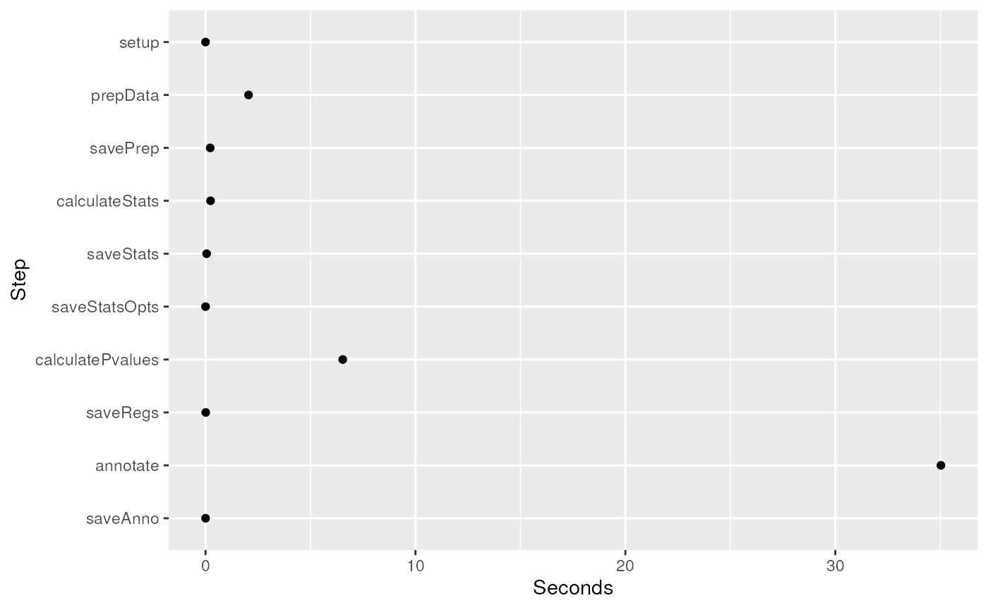
Seconds used to run each step in analyzeChr().
Merge results
Once you have analyzed each chromosome using
analyzeChr(), you can use mergeResults() to
merge the results. This function does not return an object in R but
instead creates several Rdata files with the main results from the
different chromosomes.
## Go back to the original directory
setwd(originalWd)

## Merge results from several chromosomes. In this case we only have one.
mergeResults(
    chrs = "chr21", prefix = "analysisResults",
    genomicState = genomicState$fullGenome,
    optionsStats = results$optionsStats
)
## 2026-03-31 17:43:30.079533 mergeResults: Saving options used## 2026-03-31 17:43:30.08124 Loading chromosome chr21## 2026-03-31 17:43:30.129338 mergeResults: calculating FWER## 2026-03-31 17:43:30.156528 mergeResults: Saving fullNullSummary## 2026-03-31 17:43:30.164246 mergeResults: Re-calculating the p-values## 2026-03-31 17:43:30.211696 mergeResults: Saving fullRegions## 2026-03-31 17:43:30.21702 mergeResults: assigning genomic states## 2026-03-31 17:43:30.287128 annotateRegions: counting## 2026-03-31 17:43:30.340701 annotateRegions: annotating## 2026-03-31 17:43:30.360227 mergeResults: Saving fullAnnotatedRegions## 2026-03-31 17:43:30.361939 mergeResults: Saving fullFstats## 2026-03-31 17:43:30.396506 mergeResults: Saving fullTime
## Files created by mergeResults()
dir("analysisResults", pattern = ".Rdata")
## [1] "fullAnnotatedRegions.Rdata" "fullFstats.Rdata"
## [3] "fullNullSummary.Rdata" "fullRegions.Rdata"
## [5] "fullTime.Rdata" "optionsMerge.Rdata"- fullFstats.Rdata contains a list with one element per chromosome. Per chromosome it has the F-statistics.
- fullNullSummary.Rdata is a list with the summary information from the null regions stored for each chromosome.
- fullTime.Rdata has the timing information for each chromosome as a list.
optionsMerge
For reproducibility purposes, the options used the merge the results
are stored in optionsMerge.
## Options used to merge
load(file.path("analysisResults", "optionsMerge.Rdata"))

## Contents
names(optionsMerge)
## [1] "chrs" "significantCut" "minoverlap" "mergeCall"
## [5] "cutoffFstatUsed" "optionsStats"
## Merge call
optionsMerge$mergeCall
## mergeResults(chrs = "chr21", prefix = "analysisResults", genomicState = genomicState$fullGenome,
## optionsStats = results$optionsStats)fullRegions
The main result from mergeResults() is in
fullRegions. This is a GRanges object with the
candidate DERs from all the chromosomes. It also includes the nearest
annotation metadata as well as FWER adjusted p-values (fwer)
and whether the FWER adjusted p-value is less than 0.05
(significantFWER).
## Load all the regions
load(file.path("analysisResults", "fullRegions.Rdata"))

## Metadata columns
names(mcols(fullRegions))
## [1] "value" "area"
## [3] "indexStart" "indexEnd"
## [5] "cluster" "clusterL"
## [7] "meanCoverage" "meanfetal"
## [9] "meanadult" "log2FoldChangeadultvsfetal"
## [11] "pvalues" "significant"
## [13] "qvalues" "significantQval"
## [15] "name" "annotation"
## [17] "description" "region"
## [19] "distance" "subregion"
## [21] "insideDistance" "exonnumber"
## [23] "nexons" "UTR"
## [25] "annoStrand" "geneL"
## [27] "codingL" "Geneid"
## [29] "subjectHits" "fwer"
## [31] "significantFWER"Note that analyzeChr() only has the information for a
given chromosome at a time, so mergeResults() re-calculates
the p-values and q-values using the information from all the
chromosomes.
fullAnnotatedRegions
In preparation for visually exploring the results,
mergeResults() will run annotateRegions()
which counts how many known exons, introns and intergenic segments each
candidate DER overlaps (by default with a minimum overlap of 20bp).
annotateRegions() uses a summarized version of the genome
annotation created with makeGenomicState(). For this
example, we can use the data included in derfinder
which is the summarized annotation of hg19 for chromosome 21.
## Load annotateRegions() output
load(file.path("analysisResults", "fullAnnotatedRegions.Rdata"))

## Information stored
names(fullAnnotatedRegions)
## [1] "countTable" "annotationList"
## Take a peak
lapply(fullAnnotatedRegions, head)
## $countTable
## exon intergenic intron
## 1 1 0 0
## 2 1 0 0
## 3 1 0 0
## 4 1 0 0
## 5 0 1 0
## 6 1 0 0
##
## $annotationList
## GRangesList object of length 6:
## $`1`
## GRanges object with 1 range and 4 metadata columns:
## seqnames ranges strand | theRegion tx_id
## <Rle> <IRanges> <Rle> | <character> <IntegerList>
## 4871 chr21 47609038-47611149 - | exon 73448,73449,73450,...
## tx_name gene
## <CharacterList> <IntegerList>
## 4871 uc002zij.3,uc002zik.2,uc002zil.2,... 170
## -------
## seqinfo: 1 sequence from hg19 genome
##
## $`2`
## GRanges object with 1 range and 4 metadata columns:
## seqnames ranges strand | theRegion tx_id
## <Rle> <IRanges> <Rle> | <character> <IntegerList>
## 1189 chr21 40194598-40196878 + | exon 72757,72758
## tx_name gene
## <CharacterList> <IntegerList>
## 1189 uc002yxf.3,uc002yxg.4 77
## -------
## seqinfo: 1 sequence from hg19 genome
##
## $`3`
## GRanges object with 1 range and 4 metadata columns:
## seqnames ranges strand | theRegion tx_id
## <Rle> <IRanges> <Rle> | <character> <IntegerList>
## 2965 chr21 27252861-27254082 - | exon 73066,73067,73068,...
## tx_name gene
## <CharacterList> <IntegerList>
## 2965 uc002ylz.3,uc002yma.3,uc002ymb.3,... 139
## -------
## seqinfo: 1 sequence from hg19 genome
##
## ...
## <3 more elements>ChIP-seq differential binding
As of version 1.5.27 derfinder has parameters that allow smoothing of the single base-level F-statistics before determining DERs. This allows finding differentially bounded regions (peaks) using ChIP-seq data. In general, ChIP-seq studies are smaller than RNA-seq studies which means that the single base-level F-statistics approach is well suited for differential binding analysis.
To smooth the F-statistics use smooth = TRUE in
analyzeChr(). The default smoothing function is
bumphunter::locfitByCluster() and all its parameters can be
passed specified in the call to analyzeChr(). In
particular, the minNum and bpSpan arguments
are important. We recommend setting minNum to the minimum
read length and bpSpan to the average peak length expected
in the ChIP-seq data being analyzed. Smoothing the F-statistics will
take longer but not use significantly more memory than the default
behavior. So take this into account when choosing the number of
permutations to run.
Visually explore results
Optionally, we can use the addon package derfinderPlot to visually explore the results.
To make the region level plots, we will need to extract the region
level coverage data. We can do so using getRegionCoverage()
as shown below.
## Find overlaps between regions and summarized genomic annotation
annoRegs <- annotateRegions(fullRegions, genomicState$fullGenome)
## 2026-03-31 17:43:30.788096 annotateRegions: counting## 2026-03-31 17:43:30.841819 annotateRegions: annotating
## Indeed, the result is the same because we only used chr21
identical(annoRegs, fullAnnotatedRegions)
## [1] FALSE
## Get the region coverage
regionCov <- getRegionCoverage(fullCov, fullRegions)
## 2026-03-31 17:43:30.916582 getRegionCoverage: processing chr21## 2026-03-31 17:43:30.982953 getRegionCoverage: done processing chr21
## Explore the result
head(regionCov[[1]])
## HSB113 HSB123 HSB126 HSB130 HSB135 HSB136 HSB145 HSB153 HSB159 HSB178 HSB92
## 1 0.68 0.44 0.48 0.36 0.19 2.34 1.29 1.77 2.21 2.69 1.89
## 2 0.60 0.44 0.48 0.36 0.19 2.30 1.29 1.77 2.21 2.64 1.86
## 3 0.60 0.40 0.48 0.32 0.19 2.39 1.37 1.81 2.31 2.69 1.89
## 4 0.64 0.40 0.48 0.32 0.19 2.61 1.42 1.89 2.36 2.88 1.89
## 5 0.64 0.40 0.48 0.36 0.19 2.65 1.42 1.93 2.36 2.88 1.96
## 6 0.60 0.44 0.48 0.39 0.23 2.65 1.59 1.93 2.36 2.83 1.93
## HSB97
## 1 3.57
## 2 3.60
## 3 3.60
## 4 3.60
## 5 3.70
## 6 3.70With this, we are all set to visually explore the results.
library("derfinderPlot")

## Overview of the candidate DERs in the genome
plotOverview(
    regions = fullRegions, annotation = results$annotation,
    type = "fwer"
)

suppressPackageStartupMessages(library("TxDb.Hsapiens.UCSC.hg19.knownGene"))
txdb <- TxDb.Hsapiens.UCSC.hg19.knownGene

## Base-levle coverage plots for the first 10 regions
plotRegionCoverage(
    regions = fullRegions, regionCoverage = regionCov,
    groupInfo = pheno$group, nearestAnnotation = results$annotation,
    annotatedRegions = annoRegs, whichRegions = 1:10, txdb = txdb, scalefac = 1,
    ask = FALSE
)

## Cluster plot for the first region
plotCluster(
    idx = 1, regions = fullRegions, annotation = results$annotation,
    coverageInfo = fullCov$chr21, txdb = txdb, groupInfo = pheno$group,
    titleUse = "fwer"
)
The quick start to using derfinder has example plots for the expressed regions-level approach. The vignette for derfinderPlot has even more examples.
Interactive HTML reports
We have also developed an addon package called regionReport available via Bioconductor.
The function derfinderReport() in regionReport
basically takes advantage of the results from
mergeResults() and plotting functions available in derfinderPlot
as well as other neat features from knitrBootstrap.
It then generates a customized report for single-base level F-statistics
DER finding analyses.
For results from regionMatrix() or
railMatrix() use renderReport() from regionReport.
In both cases, the resulting HTML report promotes reproducibility of the
analysis and allows you to explore in more detail the results through
some diagnostic plots.
We think that these reports are very important when you are exploring
the resulting DERs after changing a key parameter in
analyzeChr(), regionMatrix() or
railMatrix().
Check out the vignette for regionReport for example reports generated with it.
Miscellaneous features
In this section we go over some other features of derfinder which can be useful for performing feature-counts based analyses, exploring the results, or exporting data.
Feature level analysis
Similar to the expressed region-level analysis, you might be
interested in performing a feature-level analysis. More specifically,
this means getting a count matrix at the exon-level (or gene-level).
coverageToExon() allows you to get such a matrix by taking
advantage of the summarized annotation produced by
makeGenomicState().
In this example, we use the genomic state included in the package which has the information for chr21 TxDb.Hsapiens.UCSC.hg19.knownGene annotation.
## Get the exon-level matrix
system.time(exonCov <- coverageToExon(fullCov, genomicState$fullGenome, L = 76))
## class: SerialParam
## bpisup: FALSE; bpnworkers: 1; bptasks: 0; bpjobname: BPJOB
## bplog: FALSE; bpthreshold: INFO; bpstopOnError: TRUE
## bpRNGseed: ; bptimeout: NA; bpprogressbar: FALSE
## bpexportglobals: FALSE; bpexportvariables: FALSE; bpforceGC: FALSE
## bpfallback: FALSE
## bplogdir: NA
## bpresultdir: NA
## class: SerialParam
##   bpisup: FALSE; bpnworkers: 1; bptasks: 0; bpjobname: BPJOB
##   bplog: FALSE; bpthreshold: INFO; bpstopOnError: TRUE
##   bpRNGseed: ; bptimeout: NA; bpprogressbar: FALSE
##   bpexportglobals: FALSE; bpexportvariables: FALSE; bpforceGC: FALSE
##   bpfallback: FALSE
##   bplogdir: NA
##   bpresultdir: NA
## 2026-03-31 17:43:35.073735 coverageToExon: processing chromosome chr21## class: SerialParam
## bpisup: FALSE; bpnworkers: 1; bptasks: 0; bpjobname: BPJOB
## bplog: FALSE; bpthreshold: INFO; bpstopOnError: TRUE
## bpRNGseed: ; bptimeout: NA; bpprogressbar: FALSE
## bpexportglobals: FALSE; bpexportvariables: FALSE; bpforceGC: FALSE
## bpfallback: FALSE
## bplogdir: NA
## bpresultdir: NA## 2026-03-31 17:43:36.743105 coverageToExon: processing chromosome chr21## user system elapsed
## 4.939 0.103 5.042
## Dimensions of the matrix
dim(exonCov)
## [1] 2658 12
## Explore a little bit
tail(exonCov)
## HSB113 HSB123 HSB126 HSB130 HSB135 HSB136
## 4983 0.1173684 0.1382895 0.0000000 0.0000000 0.07894737 0.03947368
## 4985 4.6542105 1.4557895 1.6034210 0.7798684 1.29592103 0.72986842
## 4986 7.1510526 291.0205261 252.4892106 152.1905258 439.69500020 263.63486853
## 4988 0.0000000 0.7063158 0.7223684 0.2639474 0.48657895 0.37657895
## 4990 2.3064474 64.9423686 69.6584212 35.5769737 101.76394746 76.96736838
## 4992 0.1652632 8.1834211 9.7538158 2.4193421 10.08618420 14.41013157
## HSB145 HSB153 HSB159 HSB178 HSB92 HSB97
## 4983 5.263158e-03 0.1052632 0.04934211 0.1289474 0.03986842 0.44605264
## 4985 9.964474e-01 10.4906578 4.39013167 7.3119736 1.65184211 10.87723678
## 4986 2.345414e+02 4.5310526 10.64368415 4.9807895 11.40447366 6.23315790
## 4988 6.156579e-01 0.0000000 0.00000000 0.0000000 0.05644737 0.00000000
## 4990 5.978842e+01 1.2284210 2.67486840 0.9542105 3.98013159 1.96131579
## 4992 5.325658e+00 0.2402632 0.73039474 0.2601316 0.66907895 0.07473684With this matrix, rounded if necessary, you can proceed to use packages such as limma, DESeq2, edgeR among others.
Compare results visually
We can certainly make region-level plots using
plotRegionCoverage() or cluster plots using
plotCluster() or overview plots using
plotOveview(), all from derfinderPlot.
First we need to get the relevant annotation information.
## Annotate regions as exonic, intronic or intergenic
system.time(annoGenome <- annotateRegions(
    regionMat$chr21$regions,
    genomicState$fullGenome
))
## 2026-03-31 17:43:38.018342 annotateRegions: counting## 2026-03-31 17:43:38.078206 annotateRegions: annotating## user system elapsed
## 0.144 0.002 0.146
## Note that the genomicState object included in derfinder only has information
## for chr21 (hg19).

## Identify closest genes to regions
suppressPackageStartupMessages(library("bumphunter"))
suppressPackageStartupMessages(library("TxDb.Hsapiens.UCSC.hg19.knownGene"))
txdb <- TxDb.Hsapiens.UCSC.hg19.knownGene
genes <- annotateTranscripts(txdb)
## No annotationPackage supplied. Trying org.Hs.eg.db.## Loading required package: org.Hs.eg.db## Warning in library(package, lib.loc = lib.loc, character.only = TRUE,
## logical.return = TRUE, : there is no package called 'org.Hs.eg.db'## Could not load org.Hs.eg.db. Will continue without annotation## Getting TSS and TSE.## Getting CSS and CSE.## Warning in .set_group_names(grl, use.names, txdb, by): some group names are NAs
## or duplicated## Getting exons.## Warning in .set_group_names(grl, use.names, txdb, by): some group names are NAs
## or duplicated
system.time(annoNear <- matchGenes(regionMat$chr21$regions, genes))## user system elapsed
## 1.785 0.012 1.798Now we can proceed to use derfinderPlot to make the region-level plots for the top 100 regions.
## Identify the top regions by highest total coverage
top <- order(regionMat$chr21$regions$area, decreasing = TRUE)[1:100]

## Base-level plots for the top 100 regions with transcript information
library("derfinderPlot")
plotRegionCoverage(regionMat$chr21$regions,
    regionCoverage = regionMat$chr21$bpCoverage,
    groupInfo = pheno$group, nearestAnnotation = annoNear,
    annotatedRegions = annoGenome, whichRegions = top, scalefac = 1,
    txdb = txdb, ask = FALSE
)
However, we can alternatively use epivizr to view the candidate DERs and the region matrix results in a genome browser.
## Load epivizr, it's available from Bioconductor
library("epivizr")

## Load data to your browser
mgr <- startEpiviz()
ders_dev <- mgr$addDevice(
    fullRegions[as.logical(fullRegions$significantFWER)], "Candidate DERs"
)
ders_potential_dev <- mgr$addDevice(
    fullRegions[!as.logical(fullRegions$significantFWER)], "Potential DERs"
)
regs_dev <- mgr$addDevice(regionMat$chr21$regions, "Region Matrix")

## Go to a place you like in the genome
mgr$navigate(
    "chr21", start(regionMat$chr21$regions[top[1]]) - 100,
    end(regionMat$chr21$regions[top[1]]) + 100
)

## Stop the navigation
mgr$stopServer()
Export coverage to BigWig files
derfinder
also includes createBw() with related functions
createBwSample() and coerceGR() to export the
output of fullCoverage() to BigWig files. These functions
can be useful in the case where you start with BAM files and later on
want to save the coverage data into BigWig files, which are generally
smaller.
## Subset only the first sample
fullCovSmall <- lapply(fullCov, "[", 1)

## Export to BigWig
bw <- createBw(fullCovSmall)
## 2026-03-31 17:43:49.638177 coerceGR: coercing sample HSB113## 2026-03-31 17:43:49.67064 createBwSample: exporting bw for sample HSB113
## See the file. Note that the sample name is used to name the file.
dir(pattern = ".bw")
## [1] "HSB113.bw" "meanChr21.bw"
## Internally createBw() coerces each sample to a GRanges object before
## exporting to a BigWig file. If more than one sample was exported, the
## GRangesList would have more elements.
bw
## GRangesList object of length 1:
## $HSB113
## GRanges object with 155950 ranges and 1 metadata column:
## seqnames ranges strand | score
## <Rle> <IRanges> <Rle> | <numeric>
## chr21 chr21 9458667-9458741 * | 0.04
## chr21 chr21 9540957-9540971 * | 0.04
## chr21 chr21 9543719-9543778 * | 0.04
## chr21 chr21 9651480-9651554 * | 0.04
## chr21 chr21 9653397-9653471 * | 0.04
## ... ... ... ... . ...
## chr21 chr21 48093246-48093255 * | 0.04
## chr21 chr21 48093257-48093331 * | 0.04
## chr21 chr21 48093350-48093424 * | 0.04
## chr21 chr21 48112194-48112268 * | 0.04
## chr21 chr21 48115056-48115130 * | 0.04
## -------
## seqinfo: 1 sequence from an unspecified genomeAdvanced arguments
If you are interested in using advanced arguments in derfinder, they are described in the manual pages of each function. Some of the most common advanced arguments are:
-
chrsStyle(default isUCSC) -
verbose(by defaultTRUE).
verbose controls whether to print status updates for
nearly all the functions. chrsStyle is used to determine
the chromosome naming style and is powered by GenomeInfoDb.
Note that chrsStyle is used in any of the functions that
call extendedMapSeqlevels(). If you are working with a
different organism than Homo sapiens set the global
species option using
options(species = 'your species') with the syntax used in
names(GenomeInfoDb::genomeStyles()). If you want to disable
extendedMapSeqlevels() set chrsStyle to
NULL, which can be useful if your organism is not part of
GenomeInfoDb.
The third commonly used advanced argument is mc.cores.
It controls the number of cores to use for the functions that can run
with more than one core to speed up. In nearly all the cases, the
maximum number of cores depends on the number of chromosomes. One
notable exception is analyzeChr() where the maximum number
of cores depends on the chunksize used and the dimensions
of the data for the chromosome under study.
Note that using the ... argument allows you to specify
some of the documented arguments. For example, you might want to control
the maxClusterGap from findRegions() in the
analyzeChr() call.
Non-human data
If you are working with data from an organism that is not Homo
sapiens, then set the global options defining the
species and the chrsStyle used. For example,
if you are working with Arabidopsis Thaliana and the
NCBI naming style, then set the options using the following
code:
## Set global species and chrsStyle options
options(species = "arabidopsis_thaliana")
options(chrsStyle = "NCBI")

## Then proceed to load and analyze the data
Internally derfinder
uses extendedMapSeqlevels() to use the appropriate
chromosome naming style given a species in all functions involving
chromosome names.
Further note that the argument txdb from
analyzeChr() is passed to
bumphunter::annotateTranscripts(txdb). So if you are using
a genome different from hg19 remember to provide the
appropriate annotation data or simply use
analyzeChr(runAnnotation = FALSE).
So, in the Arabidopsis Thaliana example, your
analyzeChr() call would look like this:
## Load transcript database information
library("TxDb.Athaliana.BioMart.plantsmart28")

## Set organism options
options(species = "arabidopsis_thaliana")
options(chrsStyle = "NCBI")

## Run command with more arguments
analyzeChr(txdb = TxDb.Athaliana.BioMart.plantsmart28)
You might find the discussion Using bumphunter with non-human genomes useful.
Functions that use multiple cores
Currently, the following functions can use multiple cores, several of
which are called inside analyzeChr().
-
calculatePvalues(): 1 core per chunk of data to process. -
calculateStats(): 1 core per chunk of data to process. -
coerceGR(): 1 core per chromosome. This function is used bycreateBw(). -
coverageToExon(): 1 core per strand, then 1 core per chromosome. -
loadCoverage(): up to 1 core per tile when loading the data with GenomicFiles. Otherwise, no parallelization is used. -
fullCoverage(): 1 core per chromosome. In general, try to avoid using more than 10 cores as you might reach your maximum network speed and/or hard disk input/output seed. For the case described inloadCoverage(), you can specify how many cores to use per chromosome for the tiles using themc.cores.loadargument effectively resulting inmc.corestimesmc.cores.loadused (otherwise it’smc.coressquared). -
getRegionCoverage(): 1 core per chromosome. -
regionMatrix(): 1 core per chromosome. -
railMatrix(): 1 core per chromosome.
All parallel operations use SnowParam() from BiocParallel
when more than 1 core is being used. Otherwise,
SerialParam() is used. Note that if you prefer to specify
other types of parallelization you can do so by specifying the
BPPARAM.custom advanced argument.
Because SnowParam() requires R to load the
necessary packages on each worker, the key function
fstats.apply() was isolated in the derfinderHelper
package. This package has much faster loading speeds than derfinder
which greatly impacts performance on cases where the actual step of
calculating the F-statistics is fast.
You may prefer to use MulticoreParam() described in the
BiocParallel
vignette. In that case, when using these functions use
BPPARAM.custom = MulticoreParam(workers = x) where
x is the number of cores you want to use. Note that in some
systems, as is the case of the cluster used by derfinder’s
developers, the system tools for assessing memory usage can be
misleading, thus resulting in much higher memory loads when using
MulticoreParam() instead of the default
SnowParam().
Loading data details
Controlling loading from BAM files
If you are loading data from BAM files, you might want to specify
some criteria to decide which reads to include or not. For example, your
data might have been generated by a strand-specific protocol. You can do
so by specifying the arguments of scanBamFlag() from Rsamtools.
You can also control whether to include or exclude bases with
CIGAR string D (deletion from the reference)
by setting the advanced argument drop.D = TRUE in your
fullCoverage() or loadCoverage() call.
Unfiltered base-level coverage
Note that in most scenarios, the fullCov object
illustrated in the introductory vignette can be large in memory. When
making plots or calculating the region-level coverage, we don’t need the
full information. In such situations, it might pay off to create a
smaller version by loading only the required data. This can be achieved
using the advanced argument which to
fullCoverage() or loadCoverage().
However, it is important to consider that when reading the data from
BAM files, a read might align partially inside the region of interest.
By default such a read would be discarded and thus the base-level
coverage would be lower than what it is in reality. The advanced
argument protectWhich extends regions by 30 kbp (15 kbp
each side) to help mitigate this issue.
We can illustrate this issue with the example data from derfinder. First, we load in the data and generate some regions of interest.
## Find some regions to work with
example("loadCoverage", "derfinder")
##
## ldCvrg> datadir <- system.file("extdata", "genomeData", package = "derfinder")
##
## ldCvrg> files <- rawFiles(
## ldCvrg+ datadir = datadir, samplepatt = "*accepted_hits.bam$",
## ldCvrg+ fileterm = NULL
## ldCvrg+ )
##
## ldCvrg> ## Shorten the column names
## ldCvrg> names(files) <- gsub("_accepted_hits.bam", "", names(files))
##
## ldCvrg> ## Read and filter the data, only for 2 files
## ldCvrg> dataSmall <- loadCoverage(files = files[1:2], chr = "21", cutoff = 0)## 2026-03-31 17:43:50.084078 loadCoverage: finding chromosome lengths## 2026-03-31 17:43:50.09974 loadCoverage: loading BAM file /__w/_temp/Library/derfinder/extdata/genomeData/ERR009101_accepted_hits.bam## 2026-03-31 17:43:50.188249 loadCoverage: loading BAM file /__w/_temp/Library/derfinder/extdata/genomeData/ERR009102_accepted_hits.bam## 2026-03-31 17:43:50.23143 loadCoverage: applying the cutoff to the merged data## 2026-03-31 17:43:50.24567 filterData: originally there were 48129895 rows, now there are 454 rows. Meaning that 100 percent was filtered.##
## ldCvrg> ## Not run:
## ldCvrg> ##D ## Export to BigWig files
## ldCvrg> ##D createBw(list("chr21" = dataSmall))
## ldCvrg> ##D
## ldCvrg> ##D ## Load data from BigWig files
## ldCvrg> ##D dataSmall.bw <- loadCoverage(c(
## ldCvrg> ##D ERR009101 = "ERR009101.bw", ERR009102 =
## ldCvrg> ##D "ERR009102.bw"
## ldCvrg> ##D ), chr = "chr21")
## ldCvrg> ##D
## ldCvrg> ##D ## Compare them
## ldCvrg> ##D mapply(function(x, y) {
## ldCvrg> ##D x - y
## ldCvrg> ##D }, dataSmall$coverage, dataSmall.bw$coverage)
## ldCvrg> ##D
## ldCvrg> ##D ## Note that the only difference is the type of Rle (integer vs numeric) used
## ldCvrg> ##D ## to store the data.
## ldCvrg> ## End(Not run)
## ldCvrg>
## ldCvrg>
## ldCvrg>
## ldCvrg>
example("getRegionCoverage", "derfinder")##
## gtRgnC> ## Obtain fullCov object
## gtRgnC> fullCov <- list("21" = genomeDataRaw$coverage)
##
## gtRgnC> ## Assign chr lengths using hg19 information, use only first two regions
## gtRgnC> library("GenomeInfoDb") # for getChromInfoFromUCSC()
##
## gtRgnC> regions <- genomeRegions$regions[1:2]
##
## gtRgnC> seqlengths(regions) <- seqlengths(getChromInfoFromUCSC("hg19",
## gtRgnC+ as.Seqinfo = TRUE
## gtRgnC+ ))[
## gtRgnC+ mapSeqlevels(names(seqlengths(regions)), "UCSC")
## gtRgnC+ ]
##
## gtRgnC> ## Finally, get the region coverage
## gtRgnC> regionCov <- getRegionCoverage(fullCov = fullCov, regions = regions)## extendedMapSeqlevels: sequence names mapped from NCBI to UCSC for species homo_sapiens## 2026-03-31 17:43:50.363001 getRegionCoverage: processing chr21## 2026-03-31 17:43:50.387917 getRegionCoverage: done processing chr21Next, we load the coverage again using which but without
any padding. We can see how the coverage is not the same by looking at
the maximum coverage for each sample.
## Illustrate reading data from a set of regions
test <- loadCoverage(
    files = files, chr = "21", cutoff = NULL, which = regions,
    protectWhich = 0, fileStyle = "NCBI"
)
## extendedMapSeqlevels: sequence names mapped from UCSC to NCBI for species homo_sapiens## 2026-03-31 17:43:50.532068 loadCoverage: finding chromosome lengths## 2026-03-31 17:43:50.536755 loadCoverage: loading BAM file /__w/_temp/Library/derfinder/extdata/genomeData/ERR009101_accepted_hits.bam## 2026-03-31 17:43:50.573662 loadCoverage: loading BAM file /__w/_temp/Library/derfinder/extdata/genomeData/ERR009102_accepted_hits.bam## 2026-03-31 17:43:50.610819 loadCoverage: loading BAM file /__w/_temp/Library/derfinder/extdata/genomeData/ERR009105_accepted_hits.bam## 2026-03-31 17:43:50.648256 loadCoverage: loading BAM file /__w/_temp/Library/derfinder/extdata/genomeData/ERR009107_accepted_hits.bam## 2026-03-31 17:43:50.684815 loadCoverage: loading BAM file /__w/_temp/Library/derfinder/extdata/genomeData/ERR009108_accepted_hits.bam## 2026-03-31 17:43:50.721341 loadCoverage: loading BAM file /__w/_temp/Library/derfinder/extdata/genomeData/ERR009112_accepted_hits.bam## 2026-03-31 17:43:50.758359 loadCoverage: loading BAM file /__w/_temp/Library/derfinder/extdata/genomeData/ERR009115_accepted_hits.bam## 2026-03-31 17:43:50.794852 loadCoverage: loading BAM file /__w/_temp/Library/derfinder/extdata/genomeData/ERR009116_accepted_hits.bam## 2026-03-31 17:43:50.831373 loadCoverage: loading BAM file /__w/_temp/Library/derfinder/extdata/genomeData/ERR009131_accepted_hits.bam## 2026-03-31 17:43:50.867354 loadCoverage: loading BAM file /__w/_temp/Library/derfinder/extdata/genomeData/ERR009138_accepted_hits.bam## 2026-03-31 17:43:50.904139 loadCoverage: loading BAM file /__w/_temp/Library/derfinder/extdata/genomeData/ERR009144_accepted_hits.bam## 2026-03-31 17:43:50.941157 loadCoverage: loading BAM file /__w/_temp/Library/derfinder/extdata/genomeData/ERR009145_accepted_hits.bam## 2026-03-31 17:43:50.976687 loadCoverage: loading BAM file /__w/_temp/Library/derfinder/extdata/genomeData/ERR009148_accepted_hits.bam## 2026-03-31 17:43:51.013197 loadCoverage: loading BAM file /__w/_temp/Library/derfinder/extdata/genomeData/ERR009151_accepted_hits.bam## 2026-03-31 17:43:51.048944 loadCoverage: loading BAM file /__w/_temp/Library/derfinder/extdata/genomeData/ERR009152_accepted_hits.bam## 2026-03-31 17:43:51.087107 loadCoverage: loading BAM file /__w/_temp/Library/derfinder/extdata/genomeData/ERR009153_accepted_hits.bam## 2026-03-31 17:43:51.131069 loadCoverage: loading BAM file /__w/_temp/Library/derfinder/extdata/genomeData/ERR009159_accepted_hits.bam## 2026-03-31 17:43:51.226187 loadCoverage: loading BAM file /__w/_temp/Library/derfinder/extdata/genomeData/ERR009161_accepted_hits.bam## 2026-03-31 17:43:51.264032 loadCoverage: loading BAM file /__w/_temp/Library/derfinder/extdata/genomeData/ERR009163_accepted_hits.bam## 2026-03-31 17:43:51.30092 loadCoverage: loading BAM file /__w/_temp/Library/derfinder/extdata/genomeData/ERR009164_accepted_hits.bam## 2026-03-31 17:43:51.338335 loadCoverage: loading BAM file /__w/_temp/Library/derfinder/extdata/genomeData/ERR009167_accepted_hits.bam## 2026-03-31 17:43:51.375751 loadCoverage: loading BAM file /__w/_temp/Library/derfinder/extdata/genomeData/SRR031812_accepted_hits.bam## 2026-03-31 17:43:51.412738 loadCoverage: loading BAM file /__w/_temp/Library/derfinder/extdata/genomeData/SRR031835_accepted_hits.bam## 2026-03-31 17:43:51.447847 loadCoverage: loading BAM file /__w/_temp/Library/derfinder/extdata/genomeData/SRR031867_accepted_hits.bam## 2026-03-31 17:43:51.484721 loadCoverage: loading BAM file /__w/_temp/Library/derfinder/extdata/genomeData/SRR031868_accepted_hits.bam## 2026-03-31 17:43:51.521134 loadCoverage: loading BAM file /__w/_temp/Library/derfinder/extdata/genomeData/SRR031900_accepted_hits.bam## 2026-03-31 17:43:51.558749 loadCoverage: loading BAM file /__w/_temp/Library/derfinder/extdata/genomeData/SRR031904_accepted_hits.bam## 2026-03-31 17:43:51.59436 loadCoverage: loading BAM file /__w/_temp/Library/derfinder/extdata/genomeData/SRR031914_accepted_hits.bam## 2026-03-31 17:43:51.629504 loadCoverage: loading BAM file /__w/_temp/Library/derfinder/extdata/genomeData/SRR031936_accepted_hits.bam## 2026-03-31 17:43:51.664813 loadCoverage: loading BAM file /__w/_temp/Library/derfinder/extdata/genomeData/SRR031958_accepted_hits.bam## 2026-03-31 17:43:51.699901 loadCoverage: loading BAM file /__w/_temp/Library/derfinder/extdata/genomeData/SRR031960_accepted_hits.bam## 2026-03-31 17:43:51.735798 loadCoverage: applying the cutoff to the merged data## 2026-03-31 17:43:51.761185 filterData: originally there were 48129895 rows, now there are 48129895 rows. Meaning that 0 percent was filtered.
## Some reads were ignored and thus the coverage is lower as can be seen below:
sapply(test$coverage, max) - sapply(genomeDataRaw$coverage, max)
## ERR009101 ERR009102 ERR009105 ERR009107 ERR009108 ERR009112 ERR009115 ERR009116
## 0 0 0 0 -1 0 -1 -2
## ERR009131 ERR009138 ERR009144 ERR009145 ERR009148 ERR009151 ERR009152 ERR009153
## -2 -2 -1 -1 -3 -3 0 -3
## ERR009159 ERR009161 ERR009163 ERR009164 ERR009167 SRR031812 SRR031835 SRR031867
## -3 -3 -1 -3 -3 0 -1 0
## SRR031868 SRR031900 SRR031904 SRR031914 SRR031936 SRR031958 SRR031960
## 0 0 -1 0 0 0 0When we re-load the data using some padding to the regions, we find that the coverage matches at all the bases.
## Illustrate reading data from a set of regions

test2 <- loadCoverage(
    files = files, chr = "21", cutoff = NULL,
    which = regions, protectWhich = 3e4, fileStyle = "NCBI"
)
## extendedMapSeqlevels: sequence names mapped from UCSC to NCBI for species homo_sapiens## 2026-03-31 17:43:51.934237 loadCoverage: finding chromosome lengths## 2026-03-31 17:43:51.939001 loadCoverage: loading BAM file /__w/_temp/Library/derfinder/extdata/genomeData/ERR009101_accepted_hits.bam## 2026-03-31 17:43:51.97472 loadCoverage: loading BAM file /__w/_temp/Library/derfinder/extdata/genomeData/ERR009102_accepted_hits.bam## 2026-03-31 17:43:52.011929 loadCoverage: loading BAM file /__w/_temp/Library/derfinder/extdata/genomeData/ERR009105_accepted_hits.bam## 2026-03-31 17:43:52.04815 loadCoverage: loading BAM file /__w/_temp/Library/derfinder/extdata/genomeData/ERR009107_accepted_hits.bam## 2026-03-31 17:43:52.084076 loadCoverage: loading BAM file /__w/_temp/Library/derfinder/extdata/genomeData/ERR009108_accepted_hits.bam## 2026-03-31 17:43:52.120752 loadCoverage: loading BAM file /__w/_temp/Library/derfinder/extdata/genomeData/ERR009112_accepted_hits.bam## 2026-03-31 17:43:52.157604 loadCoverage: loading BAM file /__w/_temp/Library/derfinder/extdata/genomeData/ERR009115_accepted_hits.bam## 2026-03-31 17:43:52.233001 loadCoverage: loading BAM file /__w/_temp/Library/derfinder/extdata/genomeData/ERR009116_accepted_hits.bam## 2026-03-31 17:43:52.269705 loadCoverage: loading BAM file /__w/_temp/Library/derfinder/extdata/genomeData/ERR009131_accepted_hits.bam## 2026-03-31 17:43:52.307341 loadCoverage: loading BAM file /__w/_temp/Library/derfinder/extdata/genomeData/ERR009138_accepted_hits.bam## 2026-03-31 17:43:52.34425 loadCoverage: loading BAM file /__w/_temp/Library/derfinder/extdata/genomeData/ERR009144_accepted_hits.bam## 2026-03-31 17:43:52.383132 loadCoverage: loading BAM file /__w/_temp/Library/derfinder/extdata/genomeData/ERR009145_accepted_hits.bam## 2026-03-31 17:43:52.419806 loadCoverage: loading BAM file /__w/_temp/Library/derfinder/extdata/genomeData/ERR009148_accepted_hits.bam## 2026-03-31 17:43:52.456281 loadCoverage: loading BAM file /__w/_temp/Library/derfinder/extdata/genomeData/ERR009151_accepted_hits.bam## 2026-03-31 17:43:52.492904 loadCoverage: loading BAM file /__w/_temp/Library/derfinder/extdata/genomeData/ERR009152_accepted_hits.bam## 2026-03-31 17:43:52.530778 loadCoverage: loading BAM file /__w/_temp/Library/derfinder/extdata/genomeData/ERR009153_accepted_hits.bam## 2026-03-31 17:43:52.567112 loadCoverage: loading BAM file /__w/_temp/Library/derfinder/extdata/genomeData/ERR009159_accepted_hits.bam## 2026-03-31 17:43:52.604261 loadCoverage: loading BAM file /__w/_temp/Library/derfinder/extdata/genomeData/ERR009161_accepted_hits.bam## 2026-03-31 17:43:52.640717 loadCoverage: loading BAM file /__w/_temp/Library/derfinder/extdata/genomeData/ERR009163_accepted_hits.bam## 2026-03-31 17:43:52.677183 loadCoverage: loading BAM file /__w/_temp/Library/derfinder/extdata/genomeData/ERR009164_accepted_hits.bam## 2026-03-31 17:43:52.71431 loadCoverage: loading BAM file /__w/_temp/Library/derfinder/extdata/genomeData/ERR009167_accepted_hits.bam## 2026-03-31 17:43:52.751846 loadCoverage: loading BAM file /__w/_temp/Library/derfinder/extdata/genomeData/SRR031812_accepted_hits.bam## 2026-03-31 17:43:52.788005 loadCoverage: loading BAM file /__w/_temp/Library/derfinder/extdata/genomeData/SRR031835_accepted_hits.bam## 2026-03-31 17:43:52.824238 loadCoverage: loading BAM file /__w/_temp/Library/derfinder/extdata/genomeData/SRR031867_accepted_hits.bam## 2026-03-31 17:43:52.858759 loadCoverage: loading BAM file /__w/_temp/Library/derfinder/extdata/genomeData/SRR031868_accepted_hits.bam## 2026-03-31 17:43:52.894166 loadCoverage: loading BAM file /__w/_temp/Library/derfinder/extdata/genomeData/SRR031900_accepted_hits.bam## 2026-03-31 17:43:52.929227 loadCoverage: loading BAM file /__w/_temp/Library/derfinder/extdata/genomeData/SRR031904_accepted_hits.bam## 2026-03-31 17:43:52.965002 loadCoverage: loading BAM file /__w/_temp/Library/derfinder/extdata/genomeData/SRR031914_accepted_hits.bam## 2026-03-31 17:43:52.999303 loadCoverage: loading BAM file /__w/_temp/Library/derfinder/extdata/genomeData/SRR031936_accepted_hits.bam## 2026-03-31 17:43:53.034147 loadCoverage: loading BAM file /__w/_temp/Library/derfinder/extdata/genomeData/SRR031958_accepted_hits.bam## 2026-03-31 17:43:53.069917 loadCoverage: loading BAM file /__w/_temp/Library/derfinder/extdata/genomeData/SRR031960_accepted_hits.bam## 2026-03-31 17:43:53.144726 loadCoverage: applying the cutoff to the merged data## 2026-03-31 17:43:53.169855 filterData: originally there were 48129895 rows, now there are 48129895 rows. Meaning that 0 percent was filtered.
## Adding some padding to the regions helps get the same coverage
identical(sapply(test2$coverage, max), sapply(genomeDataRaw$coverage, max))
## [1] TRUE
## A more detailed test reveals that the coverage matches at every base
all(mapply(function(x, y) {
    identical(x, y)
}, test2$coverage, genomeDataRaw$coverage))
## [1] TRUEHow much padding you need to use will depend on your specific data set, and you might be comfortable getting approximately the same coverage values for the sake of greatly reducing the memory resources needed.
Input files in a different naming style
If you are under the case where you like to use a specific chromosome
naming style but the raw data files use another one, you might need to
use the fileStyle argument.
For example, you could be working with Homo sapiens data and
your preferred naming style is UCSC (chr1, chr2, …, chrX, chrY)
but the raw data uses NCBI style names (1, 2, …, X, Y). In that
case, use fullCoverage(fileStyle = 'NCBI') or
loadCoverage(fileStyle = 'NCBI') depending if you are
loading one chromosome or multiple at a time.
Loading data in chunks
If you prefer to do so, fullCoverage() and
loadCoverage() can load the data of a chromosome in chunks
using GenomicFiles.
This is controlled by whether you specify the tilewidth
argument.
Notice that you might run into slight coverage errors near the borders of the tiles for the same reason that was illustrated previously when loading specific regions.
This approach is not necessarily more efficient and can be
significantly time consuming if you use a small
tilewidth.
Large number of samples
If you have a large number of samples (say thousands), it might be
best to submit cluster jobs that run loadCoverage() or
fullCoverage() for only one chromosome at a time.
In the case of working with Rail
output, you can either use railMatrix() with the argument
file.cores greater than 1 or specify the advanced argument
BPPARAM.railChr to control the parallel environment used
for loading the BigWig files. Doing so, you can then submit cluster jobs
that run railMatrix() for one chromosome at a time, yet
read in the data fast. You can do all of from R by using
BPPARAM.custom and BPPARAM.railChr at the same
time where you use a BatchJobsParam() for the first
one.
Another option when working with Rail
output is to simply load the summary BigWig data (mean, median), then
define the ERs using findRegions() and write them to a BED
file. You can then use bwtool to create
the coverage matrix.
Flow charts
DER analysis flow chart
Figure @ref(fig:Figure1) illustrates how most of derfinder’s functions interact when performing a base-level differential expression analysis by calculating base-level F-statistics.

derfinder F-statistics flow chart.
Flow chart of the different processing steps (black boxes) that can
be carried out using derfinder
and the functions that perform these actions (in red). Input and output
is shown in green boxes. Functions in blue are those applied to the
results from multiple chromosomes (mergeResults() and
derfinderReport). regionReport
functions are shown in orange while derfinderPlot
functions are shown in dark purple. Purple dotted arrow marks functions
that require unfiltered base-level coverage.
analyzeChr() flow chart

analyzeChr() flow chart.
Figure @ref(fig:Figure2) shows in more detail the processing flow in
analyzeChr(), which is the main function for identifying
candidate differentially expressed regions (DERs) from the base-level
F-statistics.
Many fine-tunning arguments can be passed to
analyzeChr() to feed into the other functions. For example,
you might want to use a smaller chunksize when
pre-processing the coverage data (the default is 5 million): specially
if you have hundreds of samples.
Another useful argument is scalefac (by default it’s 32)
which controls the scaling factor to use before the log2
transformation.
Furthermore, you might want to specify maxClusterGap to
control the maximum gap between two regions before they are considered
to be part of the same cluster.
regionMatrix() flow chart

regionMatrix() flow chart.
Figure @ref(fig:Figure3) shows the functions used internally by
regionMatrix() and processing steps for identifying
expressed regions. Overall, it is much simpler than
analyzeChr(). The flow is even simpler in
railMatrix().
Base-level F-statistics projects
For each project where you will calculating base-level F-statistics,
we recommend the following organization. You might be interested in a
similar structure when using regionMatrix() if you have BAM
files. The notable exception is when you are analyzing output data from
Rail in which case you won’t be needing
this type of organization. Remember that railMatrix() is
much less computationally intensive than analyzeChr().
File organization
This is our recommended file organization when using
analyzeChr().
ProjectDir
|-derCoverageInfo
|-derAnalysis
|---analysis01
|---analysis02
We start with a main project directory that has two initial directories. One for storing the coverage data, and one for storing each analysis: you might explore different models, cutoffs or other parameters.
You can then use fullCoverage(), save the result and
also save the filtered coverage information for each chromosome
separately. Doing so will result in the following structure.
ProjectDir
|-derCoverageInfo
|---Chr1Cov.Rdata
|---Chr2Cov.Rdata
...
|---ChrYCov.Rdata
|---fullCov.Rdata
|-derAnalysis
|---analysis01
|---analysis02
Next, you can use analyzeChr() for each of the
chromosomes of a specific analysis (say analysis01). Doing so
will create several Rdata files per chromosome as shown below.
bash scripts can be useful if you wish to submit one
cluster job per chromosome. In general, you will use the same model and
group information for each chromosome, so saving the information can be
useful.
ProjectDir
|-derCoverageInfo
|---Chr1Cov.Rdata
|---Chr2Cov.Rdata
...
|---ChrYCov.Rdata
|---fullCov.Rdata
|-derAnalysis
|---analysis01
|-----models.Rdata
|-----groupInfo.Rdata
|-----chr1/
|-------chunksDir/
|-------logs/
|-------annotation.Rdata
|-------coveragePrep.Rdata
|-------fstats.Rdata
|-------optionsStats.Rdata
|-------regions.Rdata
|-------timeinfo.Rdata
|-----chr2/
...
|-----chrY/
|---analysis02
Then use mergeResults() to pool together the results
from all the chromosomes for a given analysis (here
analysis01).
ProjectDir
|-derCoverageInfo
|---Chr1Cov.Rdata
|---Chr2Cov.Rdata
...
|---ChrYCov.Rdata
|---fullCov.Rdata
|-derAnalysis
|---analysis01
|-----logs/
|-----fullAnnotatedRegions.Rdata
|-----fullFstats.Rdata
|-----fullNullSummary.Rdata
|-----fullRegions.Rdata
|-----fullTime.Rdata
|-----optionsMerge.Rdata
|-----chr1/
|-------chunksDir/
|-------logs/
|-------annotation.Rdata
|-------coveragePrep.Rdata
|-------fstats.Rdata
|-------optionsStats.Rdata
|-------regions.Rdata
|-------timeinfo.Rdata
|-----chr2/
...
|-----chrY/
|---analysis02
Finally, you might want to use derfinderReport() from
regionReport
to create a HTML report of the results.
bash scripts
If you are following our recommended file organization for a
base-level F-statistics DER finding analysis, you might be interested in
the following bash scripts templates. Note that there are
plenty of other solutions, such as writing a master R
script and using BiocParallel
to submit jobs and administer them for you. Check out the
BatchJobsParam() for more information. If you want to use
bash scripts, take a look below.
For interacting between bash and R we have
found quite useful the getopt
package. Here we include an example R script that is
controlled by a bash script which submits a job for each
chromosome to analyze for a given analysis.
The two files, derfinderAnalysis.R and derAnalysis.sh should live under the derAnalysis directory.
ProjectDir
|-derCoverageInfo
|---Chr1Cov.Rdata
|---Chr2Cov.Rdata
...
|---ChrYCov.Rdata
|---fullCov.Rdata
|-derAnalysis
|---derfinder-Analysis.R
|---derAnalysis.sh
|---analysis01
|---analysis02
Then, you can simply use:
to run analyzeChr() on all your chromosomes.
derfinder-analysis.R
## Run derfinder's analysis steps with timing info

## Load libraries
library("getopt")

## Available at http:/bioconductor.org/packages/derfinder
library("derfinder")

## Specify parameters
spec <- matrix(c(
    "DFfile", "d", 1, "character", "path to the .Rdata file with the results from loadCoverage()",
    "chr", "c", 1, "character", "Chromosome under analysis. Use X instead of chrX.",
    "mcores", "m", 1, "integer", "Number of cores",
    "verbose", "v", 2, "logical", "Print status updates",
    "help", "h", 0, "logical", "Display help"
), byrow = TRUE, ncol = 5)
opt <- getopt(spec)

## Testing the script
test <- FALSE
if (test) {
    ## Speficy it using an interactive R session and testing
    test <- TRUE
}

## Test values
if (test) {
    opt <- NULL
    opt$DFfile <- "/ProjectDir/derCoverageInfo/chr21Cov.Rdata"
    opt$chr <- "21"
    opt$mcores <- 1
    opt$verbose <- NULL
}

## if help was asked for print a friendly message
## and exit with a non-zero error code
if (!is.null(opt$help)) {
    cat(getopt(spec, usage = TRUE))
    q(status = 1)
}

## Default value for verbose = TRUE
if (is.null(opt$verbose)) opt$verbose <- TRUE

if (opt$verbose) message("Loading Rdata file with the output from loadCoverage()")
load(opt$DFfile)

## Make it easy to use the name later. Here I'm assuming the names were generated using output='auto' in loadCoverage()
eval(parse(text = paste0("data <- ", "chr", opt$chr, "CovInfo")))
eval(parse(text = paste0("rm(chr", opt$chr, "CovInfo)")))

## Just for testing purposes
if (test) {
    tmp <- data
    tmp$coverage <- tmp$coverage[1:1e6, ]
    library("IRanges")
    tmp$position[which(tmp$pos)[1e6 + 1]:length(tmp$pos)] <- FALSE
    data <- tmp
}

## Load the models
load("models.Rdata")

## Load group information
load("groupInfo.Rdata")


## Run the analysis with lowMemDir
analyzeChr(
    chr = opt$chr, coverageInfo = data, models = models,
    cutoffFstat = 1e-06, cutoffType = "theoretical", nPermute = 1000,
    seeds = seq_len(1000), maxClusterGap = 3000, groupInfo = groupInfo,
    subject = "hg19", mc.cores = opt$mcores,
    lowMemDir = file.path(tempdir(), paste0("chr", opt$chr), "chunksDir"),
    verbose = opt$verbose, chunksize = 1e5
)

## Done
if (opt$verbose) {
    print(proc.time())
    print(sessionInfo(), locale = FALSE)
}
Remember to modify the the script to fit your project.
derAnalysis.sh
#!/bin/sh

## Usage
# sh derAnalysis.sh analysis01

# Directories
MAINDIR=/ProjectDir
WDIR=${MAINDIR}/derAnalysis
DATADIR=${MAINDIR}/derCoverageInfo

# Define variables
SHORT='derA-01'
PREFIX=$1

# Construct shell files
for chrnum in 22 21 Y 20 19 18 17 16 15 14 13 12 11 10 9 8 X 7 6 5 4 3 2 1
do
    echo "Creating script for chromosome ${chrnum}"

    if [[ ${chrnum} == "Y" ]]
    then
        CORES=2
    else
        CORES=6
    fi

    chr="chr${chrnum}"
    outdir="${PREFIX}/${chr}"
    sname="${SHORT}.${PREFIX}.${chr}"
    cat > ${WDIR}/.${sname}.sh <<EOF
#!/bin/bash
#$ -cwd
#$ -m e
#$ -l mem_free=8G,h_vmem=10G,h_fsize=10G
#$ -N ${sname}
#$ -pe local ${CORES}

echo "**** Job starts ****"
date

# Create output directory
mkdir -p ${WDIR}/${outdir}
# Make logs directory
mkdir -p ${WDIR}/${outdir}/logs

# run derfinder-analysis.R
cd ${WDIR}/${PREFIX}/

# specific to our cluster
# see http://www.jhpce.jhu.edu/knowledge-base/environment-modules/
module load R/3.3.x
Rscript ${WDIR}/derfinder-analysis.R -d "${DATADIR}/${chr}Cov.Rdata" -c "${chrnum}" -m ${CORES} -v TRUE

# Move log files into the logs directory
mv ${WDIR}/${sname}.* ${WDIR}/${outdir}/logs/

echo "**** Job ends ****"
date
EOF
    call="qsub .${sname}.sh"
    $call
done
Your cluster might specify memory requirements differently and you might need to use fewer or more cores depending on your data set.
Expressed regions-level projects
If you are using regionMatrix(), an organization similar
to the one we mentioned for the single base-level F-statistics
implementation is recommended. If you have a very large number of
samples, it might be best to store the coverage data separately by
chromosome instead of a single fullCov object. This is help
with the memory load since you can then write a script for loading the
coverage data for the chromosome of interest and running
regionMatrix() on it. Once all your jobs are done, merge
the results from them.
If you are using railMatrix(), you don’t need any fancy
setup. You only need the paths to the summary files and the sample
files, all of which are assumed to be BigWig files.
Summary
We have illustrated how to identify candidate differentially
expressed regions without using annotation by using
analyzeChr(). Furthermore, we covered how to perform the
expressed region-level matrix analysis with regionMatrix()
or railMatrix(). We also highlighted other uses of the
derfinder
package.
Latter sections of this vignette covered the most commonly used advanced arguments, details on how to load data, flow charts explaining the relationships between the functions, the recommended output organization, and example shell scripts for running the analysis.
Reproducibility
This package was made possible thanks to:
- R (R Core Team, 2026)
- AnnotationDbi (Pagès, Carlson, Falcon, and Li, 2017)
- BiocParallel (Wang, Morgan, Obenchain, Lang, Thompson, and Turaga, 2025)
- bumphunter (Jaffe, Murakami, Lee, Leek, Fallin, Feinberg, and Irizarry, 2012) and (Jaffe, Murakami, Lee, Leek, Fallin, Feinberg, and Irizarry, 2012)
- derfinderHelper (Collado-Torres, Jaffe, and Leek, 2017)
- GenomeInfoDb (Arora, Morgan, Carlson, and Pagès, 2017)
- GenomicAlignments (Lawrence, Huber, Pagès, Aboyoun, Carlson, Gentleman, Morgan, and Carey, 2013)
- GenomicFeatures (Lawrence, Huber, Pagès et al., 2013)
- GenomicFiles (Bioconductor Package Maintainer, Obenchain, Love, Shepherd, and Morgan, 2025)
- GenomicRanges (Lawrence, Huber, Pagès et al., 2013)
- Hmisc (Harrell Jr, 2026)
- IRanges (Lawrence, Huber, Pagès et al., 2013)
- qvalue (Storey, Bass, Dabney, and Robinson, 2025)
- Rsamtools (Morgan, Pagès, Obenchain, and Hayden, 2026)
- rtracklayer (Lawrence, Gentleman, and Carey, 2009)
- S4Vectors (Pagès, Lawrence, and Aboyoun, 2017)
- derfinderData (Collado-Torres, Jaffe, and Leek, 2025)
- sessioninfo (Wickham, Chang, Flight, Müller, and Hester, 2025)
- ggplot2 (Wickham, 2016)
- knitr (Xie, 2014)
- BiocStyle (Oleś, 2025)
- RefManageR (McLean, 2017)
- rmarkdown (Allaire, Xie, Dervieux, McPherson, Luraschi, Ushey, Atkins, Wickham, Cheng, Chang, and Iannone, 2026)
- testthat (Wickham, 2011)
- TxDb.Hsapiens.UCSC.hg19.knownGene (Team and Maintainer, 2025)
Code for creating the vignette
## Create the vignette
library("rmarkdown")
system.time(render("derfinder-users-guide.Rmd", "BiocStyle::html_document"))

## Extract the R code
library("knitr")
knit("derfinder-users-guide.Rmd", tangle = TRUE)
## Clean up
file.remove("derfinderUsersGuideRef.bib")
## Warning in file.remove("derfinderUsersGuideRef.bib"): cannot remove file
## 'derfinderUsersGuideRef.bib', reason 'No such file or directory'## [1] FALSE
unlink("analysisResults", recursive = TRUE)
file.remove("HSB113.bw")
## [1] TRUE
file.remove("meanChr21.bw")## [1] TRUEDate the vignette was generated.
## [1] "2026-03-31 17:43:53 UTC"Wallclock time spent generating the vignette.
## Time difference of 1.588 minsR session information.
## ─ Session info ───────────────────────────────────────────────────────────────────────────────────────────────────────
##  setting  value
##  version  R Under development (unstable) (2026-03-28 r89738)
##  os       Ubuntu 24.04.4 LTS
##  system   x86_64, linux-gnu
##  ui       X11
##  language en
##  collate  en_US.UTF-8
##  ctype    en_US.UTF-8
##  tz       UTC
##  date     2026-03-31
##  pandoc   3.9.0.2 @ /usr/bin/ (via rmarkdown)
##  quarto   1.8.25 @ /usr/local/bin/quarto
##
## ─ Packages ───────────────────────────────────────────────────────────────────────────────────────────────────────────
##  package                           * version    date (UTC) lib source
##  abind                               1.4-8      2024-09-12 [1] CRAN (R 4.6.0)
##  AnnotationDbi                     * 1.73.0     2025-10-31 [1] Bioconductor 3.23 (R 4.6.0)
##  backports                           1.5.0      2024-05-23 [1] CRAN (R 4.6.0)
##  base64enc                           0.1-6      2026-02-02 [2] CRAN (R 4.7.0)
##  bibtex                              0.5.2      2026-02-03 [1] CRAN (R 4.6.0)
##  Biobase                           * 2.71.0     2025-10-30 [1] Bioconductor 3.23 (R 4.6.0)
##  BiocGenerics                      * 0.57.0     2025-10-30 [1] Bioconductor 3.23 (R 4.6.0)
##  BiocIO                              1.21.0     2025-10-30 [1] Bioconductor 3.23 (R 4.6.0)
##  BiocManager                         1.30.27    2025-11-14 [2] CRAN (R 4.7.0)
##  BiocParallel                        1.45.0     2025-10-30 [1] Bioconductor 3.23 (R 4.6.0)
##  BiocStyle                         * 2.39.0     2025-10-30 [1] Bioconductor 3.23 (R 4.6.0)
##  Biostrings                          2.79.5     2026-03-06 [1] Bioconductor 3.23 (R 4.7.0)
##  bit                                 4.6.0      2025-03-06 [1] CRAN (R 4.6.0)
##  bit64                               4.6.0-1    2025-01-16 [1] CRAN (R 4.6.0)
##  bitops                              1.0-9      2024-10-03 [1] CRAN (R 4.6.0)
##  blob                                1.3.0      2026-01-14 [1] CRAN (R 4.6.0)
##  bookdown                            0.46       2025-12-05 [1] CRAN (R 4.6.0)
##  BSgenome                            1.79.1     2025-11-04 [1] Bioconductor 3.23 (R 4.6.0)
##  bslib                               0.10.0     2026-01-26 [2] CRAN (R 4.7.0)
##  bumphunter                        * 1.53.0     2025-11-04 [1] Bioconductor 3.23 (R 4.6.0)
##  cachem                              1.1.0      2024-05-16 [2] CRAN (R 4.7.0)
##  checkmate                           2.3.4      2026-02-03 [1] CRAN (R 4.6.0)
##  cigarillo                           1.1.0      2025-10-31 [1] Bioconductor 3.23 (R 4.6.0)
##  cli                                 3.6.5      2025-04-23 [2] CRAN (R 4.7.0)
##  cluster                             2.1.8.2    2026-02-05 [3] CRAN (R 4.7.0)
##  codetools                           0.2-20     2024-03-31 [3] CRAN (R 4.7.0)
##  colorspace                          2.1-2      2025-09-22 [1] CRAN (R 4.6.0)
##  crayon                              1.5.3      2024-06-20 [2] CRAN (R 4.7.0)
##  curl                                7.0.0      2025-08-19 [2] CRAN (R 4.7.0)
##  data.table                          1.18.2.1   2026-01-27 [1] CRAN (R 4.6.0)
##  DBI                                 1.3.0      2026-02-25 [1] CRAN (R 4.7.0)
##  DelayedArray                        0.37.0     2025-10-31 [1] Bioconductor 3.23 (R 4.6.0)
##  derfinder                         * 1.45.0     2026-03-31 [1] Bioconductor
##  derfinderData                     * 2.29.0     2025-10-30 [1] Bioconductor 3.23 (R 4.6.0)
##  derfinderHelper                     1.45.0     2025-10-31 [1] Bioconductor 3.23 (R 4.6.0)
##  desc                                1.4.3      2023-12-10 [2] CRAN (R 4.7.0)
##  DESeq2                            * 1.51.7     2026-03-13 [1] Bioconductor 3.23 (R 4.7.0)
##  dichromat                           2.0-0.1    2022-05-02 [1] CRAN (R 4.6.0)
##  digest                              0.6.39     2025-11-19 [2] CRAN (R 4.7.0)
##  doRNG                               1.8.6.3    2026-02-05 [1] CRAN (R 4.6.0)
##  dplyr                               1.2.0      2026-02-03 [1] CRAN (R 4.6.0)
##  evaluate                            1.0.5      2025-08-27 [2] CRAN (R 4.7.0)
##  farver                              2.1.2      2024-05-13 [1] CRAN (R 4.6.0)
##  fastmap                             1.2.0      2024-05-15 [2] CRAN (R 4.7.0)
##  foreach                           * 1.5.2      2022-02-02 [1] CRAN (R 4.6.0)
##  foreign                             0.8-91     2026-01-29 [3] CRAN (R 4.7.0)
##  Formula                             1.2-5      2023-02-24 [1] CRAN (R 4.6.0)
##  fs                                  2.0.1      2026-03-24 [2] CRAN (R 4.7.0)
##  generics                          * 0.1.4      2025-05-09 [1] CRAN (R 4.6.0)
##  GenomeInfoDb                      * 1.47.2     2025-12-04 [1] Bioconductor 3.23 (R 4.6.0)
##  GenomicAlignments                   1.47.0     2025-10-31 [1] Bioconductor 3.23 (R 4.6.0)
##  GenomicFeatures                   * 1.63.1     2025-11-04 [1] Bioconductor 3.23 (R 4.6.0)
##  GenomicFiles                        1.47.0     2025-11-04 [1] Bioconductor 3.23 (R 4.6.0)
##  GenomicRanges                     * 1.63.1     2025-12-08 [1] Bioconductor 3.23 (R 4.6.0)
##  ggplot2                           * 4.0.2      2026-02-03 [1] CRAN (R 4.6.0)
##  glue                                1.8.0      2024-09-30 [2] CRAN (R 4.7.0)
##  gridExtra                           2.3        2017-09-09 [1] CRAN (R 4.6.0)
##  gtable                              0.3.6      2024-10-25 [1] CRAN (R 4.6.0)
##  Hmisc                               5.2-5      2026-01-09 [1] CRAN (R 4.6.0)
##  htmlTable                           2.4.3      2024-07-21 [1] CRAN (R 4.6.0)
##  htmltools                           0.5.9      2025-12-04 [2] CRAN (R 4.7.0)
##  htmlwidgets                         1.6.4      2023-12-06 [2] CRAN (R 4.7.0)
##  httr                                1.4.8      2026-02-13 [1] CRAN (R 4.7.0)
##  IRanges                           * 2.45.0     2025-10-31 [1] Bioconductor 3.23 (R 4.6.0)
##  iterators                         * 1.0.14     2022-02-05 [1] CRAN (R 4.6.0)
##  jquerylib                           0.1.4      2021-04-26 [2] CRAN (R 4.7.0)
##  jsonlite                            2.0.0      2025-03-27 [2] CRAN (R 4.7.0)
##  KEGGREST                            1.51.1     2025-11-17 [1] Bioconductor 3.23 (R 4.6.0)
##  knitr                             * 1.51       2025-12-20 [2] CRAN (R 4.7.0)
##  labeling                            0.4.3      2023-08-29 [1] CRAN (R 4.6.0)
##  lattice                             0.22-9     2026-02-09 [3] CRAN (R 4.7.0)
##  lifecycle                           1.0.5      2026-01-08 [2] CRAN (R 4.7.0)
##  limma                             * 3.67.0     2025-10-30 [1] Bioconductor 3.23 (R 4.6.0)
##  locfit                            * 1.5-9.12   2025-03-05 [1] CRAN (R 4.6.0)
##  lubridate                           1.9.5      2026-02-04 [1] CRAN (R 4.6.0)
##  magrittr                            2.0.4      2025-09-12 [2] CRAN (R 4.7.0)
##  Matrix                              1.7-5      2026-03-21 [3] CRAN (R 4.7.0)
##  MatrixGenerics                    * 1.23.0     2025-10-30 [1] Bioconductor 3.23 (R 4.6.0)
##  matrixStats                       * 1.5.0      2025-01-07 [1] CRAN (R 4.6.0)
##  memoise                             2.0.1      2021-11-26 [2] CRAN (R 4.7.0)
##  nnet                                7.3-20     2025-01-01 [3] CRAN (R 4.7.0)
##  otel                                0.2.0      2025-08-29 [2] CRAN (R 4.7.0)
##  pillar                              1.11.1     2025-09-17 [2] CRAN (R 4.7.0)
##  pkgconfig                           2.0.3      2019-09-22 [2] CRAN (R 4.7.0)
##  pkgdown                             2.2.0.9000 2026-03-31 [1] Github (r-lib/pkgdown@a6abe43)
##  plyr                                1.8.9      2023-10-02 [1] CRAN (R 4.6.0)
##  png                                 0.1-9      2026-03-15 [1] CRAN (R 4.7.0)
##  qvalue                              2.43.0     2025-10-30 [1] Bioconductor 3.23 (R 4.6.0)
##  R6                                  2.6.1      2025-02-15 [2] CRAN (R 4.7.0)
##  ragg                                1.5.2      2026-03-23 [2] CRAN (R 4.7.0)
##  RColorBrewer                        1.1-3      2022-04-03 [1] CRAN (R 4.6.0)
##  Rcpp                                1.1.1      2026-01-10 [2] CRAN (R 4.7.0)
##  RCurl                               1.98-1.18  2026-03-21 [1] CRAN (R 4.7.0)
##  RefManageR                        * 1.4.0      2022-09-30 [1] CRAN (R 4.6.0)
##  reshape2                            1.4.5      2025-11-12 [1] CRAN (R 4.6.0)
##  restfulr                            0.0.16     2025-06-27 [1] CRAN (R 4.6.0)
##  rjson                               0.2.23     2024-09-16 [1] CRAN (R 4.6.0)
##  rlang                               1.1.7      2026-01-09 [2] CRAN (R 4.7.0)
##  rmarkdown                           2.31       2026-03-26 [2] CRAN (R 4.7.0)
##  rngtools                            1.5.2      2021-09-20 [1] CRAN (R 4.6.0)
##  rpart                               4.1.27     2026-03-27 [3] CRAN (R 4.7.0)
##  Rsamtools                           2.27.1     2026-03-08 [1] Bioconductor 3.23 (R 4.7.0)
##  RSQLite                             2.4.6      2026-02-06 [1] CRAN (R 4.6.0)
##  rstudioapi                          0.18.0     2026-01-16 [2] CRAN (R 4.7.0)
##  rtracklayer                         1.71.3     2025-12-14 [1] Bioconductor 3.23 (R 4.6.0)
##  S4Arrays                            1.11.1     2025-11-25 [1] Bioconductor 3.23 (R 4.6.0)
##  S4Vectors                         * 0.49.0     2025-10-30 [1] Bioconductor 3.23 (R 4.6.0)
##  S7                                  0.2.1      2025-11-14 [1] CRAN (R 4.6.0)
##  sass                                0.4.10     2025-04-11 [2] CRAN (R 4.7.0)
##  scales                              1.4.0      2025-04-24 [1] CRAN (R 4.6.0)
##  Seqinfo                           * 1.1.0      2025-10-31 [1] Bioconductor 3.23 (R 4.6.0)
##  sessioninfo                       * 1.2.3      2025-02-05 [2] CRAN (R 4.7.0)
##  SparseArray                         1.11.12    2026-03-30 [1] Bioconductor 3.23 (R 4.7.0)
##  statmod                             1.5.1      2025-10-09 [1] CRAN (R 4.6.0)
##  stringi                             1.8.7      2025-03-27 [2] CRAN (R 4.7.0)
##  stringr                             1.6.0      2025-11-04 [2] CRAN (R 4.7.0)
##  SummarizedExperiment              * 1.41.1     2026-02-06 [1] Bioconductor 3.23 (R 4.6.0)
##  systemfonts                         1.3.2      2026-03-05 [2] CRAN (R 4.7.0)
##  textshaping                         1.0.5      2026-03-06 [2] CRAN (R 4.7.0)
##  tibble                              3.3.1      2026-01-11 [2] CRAN (R 4.7.0)
##  tidyselect                          1.2.1      2024-03-11 [1] CRAN (R 4.6.0)
##  timechange                          0.4.0      2026-01-29 [1] CRAN (R 4.6.0)
##  TxDb.Hsapiens.UCSC.hg19.knownGene * 3.22.1     2026-02-11 [1] Bioconductor
##  UCSC.utils                          1.7.1      2025-12-09 [1] Bioconductor 3.23 (R 4.6.0)
##  VariantAnnotation                   1.57.1     2025-12-18 [1] Bioconductor 3.23 (R 4.6.0)
##  vctrs                               0.7.2      2026-03-21 [2] CRAN (R 4.7.0)
##  withr                               3.0.2      2024-10-28 [2] CRAN (R 4.7.0)
##  xfun                                0.57       2026-03-20 [2] CRAN (R 4.7.0)
##  XML                                 3.99-0.23  2026-03-20 [1] CRAN (R 4.7.0)
##  xml2                                1.5.2      2026-01-17 [2] CRAN (R 4.7.0)
##  XVector                             0.51.0     2025-10-31 [1] Bioconductor 3.23 (R 4.6.0)
##  yaml                                2.3.12     2025-12-10 [2] CRAN (R 4.7.0)
##
##  [1] /__w/_temp/Library
##  [2] /usr/local/lib/R/site-library
##  [3] /usr/local/lib/R/library
##  * ── Packages attached to the search path.
##
## ──────────────────────────────────────────────────────────────────────────────────────────────────────────────────────
Bibliography
This vignette was generated using BiocStyle (Oleś, 2025) with knitr (Xie, 2014) and rmarkdown (Allaire, Xie, Dervieux et al., 2026) running behind the scenes.
Citations made with RefManageR (McLean, 2017).
[1] J. Allaire, Y. Xie, C. Dervieux, et al. rmarkdown: Dynamic Documents for R. R package version 2.31. 2026. URL: https://github.com/rstudio/rmarkdown.
[2] S. Arora, M. Morgan, M. Carlson, et al. GenomeInfoDb: Utilities for manipulating chromosome and other ‘seqname’ identifiers. 2017. DOI: 10.18129/B9.bioc.GenomeInfoDb.
[3] Bioconductor Package Maintainer, V. Obenchain, M. Love, et al. GenomicFiles: Distributed computing by file or by range. R package version 1.47.0. 2025. DOI: 10.18129/B9.bioc.GenomicFiles. URL: https://bioconductor.org/packages/GenomicFiles.
[4] BrainSpan. “Atlas of the Developing Human Brain [Internet]. Funded by ARRA Awards 1RC2MH089921-01, 1RC2MH090047-01, and 1RC2MH089929-01.” 2011. URL: http://www.brainspan.org/.
[5] L. Collado-Torres, A. E. Jaffe, and J. T. Leek. derfinderHelper: derfinder helper package. https://github.com/leekgroup/derfinderHelper - R package version 1.45.0. 2017. DOI: 10.18129/B9.bioc.derfinderHelper. URL: http://www.bioconductor.org/packages/derfinderHelper.
[6] L. Collado-Torres, A. Jaffe, and J. Leek. derfinderData: Processed BigWigs from BrainSpan for examples. R package version 2.29.0. 2025. DOI: 10.18129/B9.bioc.derfinderData. URL: https://bioconductor.org/packages/derfinderData.
[7] A. C. Frazee, S. Sabunciyan, K. D. Hansen, et al. “Differential expression analysis of RNA-seq data at single-base resolution”. In: Biostatistics 15 (3) (2014), pp. 413-426. DOI: 10.1093/biostatistics/kxt053. URL: http://biostatistics.oxfordjournals.org/content/15/3/413.long.
[8] F. Harrell Jr. Hmisc: Harrell Miscellaneous. R package version 5.2-5. 2026. DOI: 10.32614/CRAN.package.Hmisc. URL: https://CRAN.R-project.org/package=Hmisc.
[9] A. E. Jaffe, P. Murakami, H. Lee, et al. “Bump hunting to identify differentially methylated regions in epigenetic epidemiology studies”. In: International journal of epidemiology 41.1 (2012), pp. 200–209. DOI: 10.1093/ije/dyr238.
[10] A. E. Jaffe, P. Murakami, H. Lee, et al. “Bump hunting to identify differentially methylated regions in epigenetic epidemiology studies”. In: International Journal of Epidemiology (2012).
[11] M. Lawrence, R. Gentleman, and V. Carey. “rtracklayer: an R package for interfacing with genome browsers”. In: Bioinformatics 25 (2009), pp. 1841-1842. DOI: 10.1093/bioinformatics/btp328. URL: http://bioinformatics.oxfordjournals.org/content/25/14/1841.abstract.
[12] M. Lawrence, W. Huber, H. Pagès, et al. “Software for Computing and Annotating Genomic Ranges”. In: PLoS Computational Biology 9 (8 2013). DOI: 10.1371/journal.pcbi.1003118. URL: http://www.ploscompbiol.org/article/info%3Adoi%2F10.1371%2Fjournal.pcbi.1003118}.
[13] M. W. McLean. “RefManageR: Import and Manage BibTeX and BibLaTeX References in R”. In: The Journal of Open Source Software (2017). DOI: 10.21105/joss.00338.
[14] M. Morgan, H. Pagès, V. Obenchain, et al. Rsamtools: Binary alignment (BAM), FASTA, variant call (BCF), and tabix file import. R package version 2.27.1. 2026. DOI: 10.18129/B9.bioc.Rsamtools. URL: https://bioconductor.org/packages/Rsamtools.
[15] A. Oleś. BiocStyle: Standard styles for vignettes and other Bioconductor documents. R package version 2.39.0. 2025. DOI: 10.18129/B9.bioc.BiocStyle. URL: https://bioconductor.org/packages/BiocStyle.
[16] H. Pagès, M. Carlson, S. Falcon, et al. AnnotationDbi: Annotation Database Interface. 2017. DOI: 10.18129/B9.bioc.AnnotationDbi.
[17] H. Pagès, M. Lawrence, and P. Aboyoun. S4Vectors: S4 implementation of vector-like and list-like objects. 2017. DOI: 10.18129/B9.bioc.S4Vectors.
[18] R Core Team. R: A Language and Environment for Statistical Computing. R Foundation for Statistical Computing (ROR: <https://ror.org/05qewa988>;). Vienna, Austria, 2026. DOI: 10.32614/R.manuals. URL: https://www.R-project.org/.
[19] J. D. Storey, A. J. Bass, A. Dabney, et al. qvalue: Q-value estimation for false discovery rate control. R package version 2.43.0. 2025. DOI: 10.18129/B9.bioc.qvalue. URL: https://bioconductor.org/packages/qvalue.
[20] B. C. Team and B. P. Maintainer. TxDb.Hsapiens.UCSC.hg19.knownGene: Annotation package for TxDb object(s). R package version 3.22.1. 2025.
[21] J. Wang, M. Morgan, V. Obenchain, et al. BiocParallel: Bioconductor facilities for parallel evaluation. R package version 1.45.0. 2025. DOI: 10.18129/B9.bioc.BiocParallel. URL: https://bioconductor.org/packages/BiocParallel.
[22] H. Wickham. ggplot2: Elegant Graphics for Data Analysis. Springer-Verlag New York, 2016. ISBN: 978-3-319-24277-4. URL: https://ggplot2.tidyverse.org.
[23] H. Wickham. “testthat: Get Started with Testing”. In: The R Journal 3 (2011), pp. 5–10. URL: https://journal.r-project.org/articles/RJ-2011-002/.
[24] H. Wickham, W. Chang, R. Flight, et al. sessioninfo: R Session Information. R package version 1.2.3. 2025. DOI: 10.32614/CRAN.package.sessioninfo. URL: https://CRAN.R-project.org/package=sessioninfo.
[25] Y. Xie. “knitr: A Comprehensive Tool for Reproducible Research in R”. In: Implementing Reproducible Computational Research. Ed. by V. Stodden, F. Leisch and R. D. Peng. ISBN 978-1466561595. Chapman and Hall/CRC, 2014.