10 Differential gene expression analysis with limma

Instructor: Leo

10.1 SRP045638 data

We’ll use data from https://www.ncbi.nlm.nih.gov/sra/?term=SRP045638 processed and made available through the recount3 project. First, we need to download the data with the same commands we saw earlier.

library("recount3")

human_projects <- available_projects()
#> 2023-07-11 22:08:37.284382 caching file sra.recount_project.MD.gz.
#> 2023-07-11 22:08:37.649216 caching file gtex.recount_project.MD.gz.
#> 2023-07-11 22:08:38.020325 caching file tcga.recount_project.MD.gz.

rse_gene_SRP045638 <- create_rse(
    subset(
        human_projects,
        project == "SRP045638" & project_type == "data_sources"
    )
)
#> 2023-07-11 22:08:41.897366 downloading and reading the metadata.
#> 2023-07-11 22:08:42.144861 caching file sra.sra.SRP045638.MD.gz.
#> adding rname 'http://duffel.rail.bio/recount3/human/data_sources/sra/metadata/38/SRP045638/sra.sra.SRP045638.MD.gz'
#> 2023-07-11 22:08:43.384775 caching file sra.recount_project.SRP045638.MD.gz.
#> adding rname 'http://duffel.rail.bio/recount3/human/data_sources/sra/metadata/38/SRP045638/sra.recount_project.SRP045638.MD.gz'
#> 2023-07-11 22:08:44.408273 caching file sra.recount_qc.SRP045638.MD.gz.
#> adding rname 'http://duffel.rail.bio/recount3/human/data_sources/sra/metadata/38/SRP045638/sra.recount_qc.SRP045638.MD.gz'
#> 2023-07-11 22:08:45.475622 caching file sra.recount_seq_qc.SRP045638.MD.gz.
#> adding rname 'http://duffel.rail.bio/recount3/human/data_sources/sra/metadata/38/SRP045638/sra.recount_seq_qc.SRP045638.MD.gz'
#> 2023-07-11 22:08:46.506184 caching file sra.recount_pred.SRP045638.MD.gz.
#> adding rname 'http://duffel.rail.bio/recount3/human/data_sources/sra/metadata/38/SRP045638/sra.recount_pred.SRP045638.MD.gz'
#> 2023-07-11 22:08:47.399719 downloading and reading the feature information.
#> 2023-07-11 22:08:47.62401 caching file human.gene_sums.G026.gtf.gz.
#> 2023-07-11 22:08:48.398253 downloading and reading the counts: 66 samples across 63856 features.
#> 2023-07-11 22:08:48.750068 caching file sra.gene_sums.SRP045638.G026.gz.
#> adding rname 'http://duffel.rail.bio/recount3/human/data_sources/sra/gene_sums/38/SRP045638/sra.gene_sums.SRP045638.G026.gz'
#> 2023-07-11 22:08:50.244939 constructing the RangedSummarizedExperiment (rse) object.
assay(rse_gene_SRP045638, "counts") <- compute_read_counts(rse_gene_SRP045638)

Now that we have the data and have computed the read counts (which will be needed for downstream analyses), we can use expand_sra_attributes() to make it easier to use the sample information in downstream analyses. However, we have to resolve some issues with this data first.

## Can you notice the problem with the sample information?
rse_gene_SRP045638$sra.sample_attributes[1:3]
#> [1] "age;;67.78|biomaterial_provider;;LIBD|BioSampleModel;;Human|dev_stage;;Fetal|disease;;Control|Fraction;;total|isolate;;DLPFC|race;;AA|RIN;;8.3|sex;;female|tissue;;DLPFC"
#> [2] "age;;40.42|biomaterial_provider;;LIBD|BioSampleModel;;Human|disease;;Control|Fraction;;total|isolate;;DLPFC|race;;AA|RIN;;8.4|sex;;male|tissue;;DLPFC"                   
#> [3] "age;;41.58|biomaterial_provider;;LIBD|BioSampleModel;;Human|disease;;control|Fraction;;total|isolate;;R2869|race;;AA|RIN;;8.7|sex;;male|tissue;;DLPFC"

Lets resolve the issue we detected with this sample information. We’ll resolve this by eliminating some information that is only present in a subset of samples and that we don’t need.

rse_gene_SRP045638$sra.sample_attributes <- gsub("dev_stage;;Fetal\\|", "", rse_gene_SRP045638$sra.sample_attributes)
rse_gene_SRP045638$sra.sample_attributes[1:3]
#> [1] "age;;67.78|biomaterial_provider;;LIBD|BioSampleModel;;Human|disease;;Control|Fraction;;total|isolate;;DLPFC|race;;AA|RIN;;8.3|sex;;female|tissue;;DLPFC"
#> [2] "age;;40.42|biomaterial_provider;;LIBD|BioSampleModel;;Human|disease;;Control|Fraction;;total|isolate;;DLPFC|race;;AA|RIN;;8.4|sex;;male|tissue;;DLPFC"  
#> [3] "age;;41.58|biomaterial_provider;;LIBD|BioSampleModel;;Human|disease;;control|Fraction;;total|isolate;;R2869|race;;AA|RIN;;8.7|sex;;male|tissue;;DLPFC"

Now we can continue our work using similar code from the one we used earlier.

rse_gene_SRP045638 <- expand_sra_attributes(rse_gene_SRP045638)

colData(rse_gene_SRP045638)[
    ,
    grepl("^sra_attribute", colnames(colData(rse_gene_SRP045638)))
]
#> DataFrame with 66 rows and 10 columns
#>            sra_attribute.age sra_attribute.biomaterial_provider sra_attribute.BioSampleModel sra_attribute.disease
#>                  <character>                        <character>                  <character>           <character>
#> SRR2071341             67.78                               LIBD                        Human               Control
#> SRR2071345             40.42                               LIBD                        Human               Control
#> SRR2071346             41.58                               LIBD                        Human               control
#> SRR2071347             44.17                               LIBD                        Human               control
#>            sra_attribute.Fraction sra_attribute.isolate sra_attribute.race sra_attribute.RIN sra_attribute.sex
#>                       <character>           <character>        <character>       <character>       <character>
#> SRR2071341                  total                 DLPFC                 AA               8.3            female
#> SRR2071345                  total                 DLPFC                 AA               8.4              male
#> SRR2071346                  total                 R2869                 AA               8.7              male
#> SRR2071347                  total                 R3098                 AA               5.3            female
#>            sra_attribute.tissue
#>                     <character>
#> SRR2071341                DLPFC
#> SRR2071345                DLPFC
#> SRR2071346                DLPFC
#> SRR2071347                DLPFC
#>  [ reached getOption("max.print") -- omitted 7 rows ]

As well use the sampel information for building our statistical model, it will important that we make sure that it is on the correct format R expects later on.

## Recast character vectors into numeric or factor ones
rse_gene_SRP045638$sra_attribute.age <- as.numeric(rse_gene_SRP045638$sra_attribute.age)
rse_gene_SRP045638$sra_attribute.disease <- factor(tolower(rse_gene_SRP045638$sra_attribute.disease))
rse_gene_SRP045638$sra_attribute.RIN <- as.numeric(rse_gene_SRP045638$sra_attribute.RIN)
rse_gene_SRP045638$sra_attribute.sex <- factor(rse_gene_SRP045638$sra_attribute.sex)

## Summary of our variables of interest
summary(as.data.frame(colData(rse_gene_SRP045638)[
    ,
    grepl("^sra_attribute.[age|disease|RIN|sex]", colnames(colData(rse_gene_SRP045638)))
]))
#>  sra_attribute.age sra_attribute.disease sra_attribute.isolate sra_attribute.RIN sra_attribute.sex
#>  Min.   :-0.4986   control:66            Length:66             Min.   :5.30      female:22        
#>  1st Qu.: 0.3424                         Class :character      1st Qu.:8.00      male  :44        
#>  Median :14.9000                         Mode  :character      Median :8.30                       
#>  Mean   :22.6286                                               Mean   :8.15                       
#>  3rd Qu.:41.2900                                               3rd Qu.:8.70                       
#>  Max.   :73.9100                                               Max.   :9.60

We’ll now create a few variables from this sample information so we can use them in our analysis.

## We'll want to look for differences between prenatal and postnatal samples
rse_gene_SRP045638$prenatal <- factor(ifelse(rse_gene_SRP045638$sra_attribute.age < 0, "prenatal", "postnatal"))
table(rse_gene_SRP045638$prenatal)
#> 
#> postnatal  prenatal 
#>        56        10

## http://rna.recount.bio/docs/quality-check-fields.html
rse_gene_SRP045638$assigned_gene_prop <- rse_gene_SRP045638$recount_qc.gene_fc_count_all.assigned / rse_gene_SRP045638$recount_qc.gene_fc_count_all.total
summary(rse_gene_SRP045638$assigned_gene_prop)
#>    Min. 1st Qu.  Median    Mean 3rd Qu.    Max. 
#>  0.1942  0.7004  0.7591  0.7170  0.7991  0.8493
with(colData(rse_gene_SRP045638), plot(assigned_gene_prop, sra_attribute.RIN))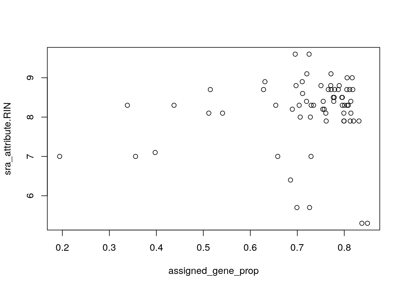


## Hm... lets check if there is a difference between these two groups
with(colData(rse_gene_SRP045638), tapply(assigned_gene_prop, prenatal, summary))
#> $postnatal
#>    Min. 1st Qu.  Median    Mean 3rd Qu.    Max. 
#>  0.1942  0.7072  0.7719  0.7179  0.8017  0.8493 
#> 
#> $prenatal
#>    Min. 1st Qu.  Median    Mean 3rd Qu.    Max. 
#>  0.6856  0.7004  0.7088  0.7116  0.7259  0.7347

We can next drop some samples that we consider of low quality as well as genes that have low expression levels.

## Lets save our full object for now in case we change our minds later on
rse_gene_SRP045638_unfiltered <- rse_gene_SRP045638

## Lets drop some bad samples. On a real analysis, you would likely use
## some statistical method for identifying outliers such as scuttle::isOutlier()
hist(rse_gene_SRP045638$assigned_gene_prop)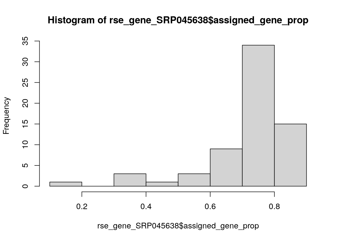

table(rse_gene_SRP045638$assigned_gene_prop < 0.3)
#> 
#> FALSE  TRUE 
#>    65     1
rse_gene_SRP045638 <- rse_gene_SRP045638[, rse_gene_SRP045638$assigned_gene_prop > 0.3]

## Lets compute the mean expression levels.
##
## Note: in a real analysis we would likely do this with RPKMs or CPMs instead
## of counts. That is, we would use one of the following options:
# edgeR::filterByExpr() https://bioconductor.org/packages/edgeR/ https://rdrr.io/bioc/edgeR/man/filterByExpr.html
# genefilter::genefilter() https://bioconductor.org/packages/genefilter/ https://rdrr.io/bioc/genefilter/man/genefilter.html
# jaffelab::expression_cutoff() http://research.libd.org/jaffelab/reference/expression_cutoff.html
#
gene_means <- rowMeans(assay(rse_gene_SRP045638, "counts"))
summary(gene_means)
#>      Min.   1st Qu.    Median      Mean   3rd Qu.      Max. 
#>       0.0       0.1       2.5     815.2     170.2 1362047.9

## We can now drop genes with low expression levels
rse_gene_SRP045638 <- rse_gene_SRP045638[gene_means > 0.1, ]

## Final dimensions of our RSE object
dim(rse_gene_SRP045638)
#> [1] 46929    65

## Percent of genes that we retained:
round(nrow(rse_gene_SRP045638) / nrow(rse_gene_SRP045638_unfiltered) * 100, 2)
#> [1] 73.49

We are now ready to continue with the differential expression analysis. Well, almost! 😅

10.2 Data normalization

Read the A hypothetical scenario in one of the edgeR papers https://genomebiology.biomedcentral.com/articles/10.1186/gb-2010-11-3-r25#Sec2 to understand the concept of composition bias.
This concept is still relevant nowadays with single cell RNA-seq (scRNA-seq) data as you can see at http://bioconductor.org/books/3.16/OSCA.multisample/multi-sample-comparisons.html#performing-the-de-analysis. In that chapter they describe a series of steps for re-using bulk RNA-seq methods with scRNA-seq data.

## Use edgeR::calcNormFactors() to address the composition bias
library("edgeR")
dge <- DGEList(
    counts = assay(rse_gene_SRP045638, "counts"),
    genes = rowData(rse_gene_SRP045638)
)
dge <- calcNormFactors(dge)

10.3 Differential expression

First of all, lets define our differential expression model. Typically, we would explore the data more to check that there are no other quality control issues with our samples and to explore in more detail the relationship between our sample phenotype variables.

library("ggplot2")
ggplot(as.data.frame(colData(rse_gene_SRP045638)), aes(y = assigned_gene_prop, x = prenatal)) +
    geom_boxplot() +
    theme_bw(base_size = 20) +
    ylab("Assigned Gene Prop") +
    xlab("Age Group")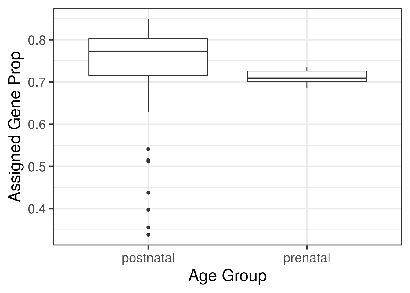

For example, we would explore the contribution of different variables to the gene expression variability we observe using the variancePartition and scater Bioconductor packages, among others. We’ll do more of this tomorrow but you can also check these LIBD rstats club notes.

For now, we’ll use the following stastistical model.

mod <- model.matrix(~ prenatal + sra_attribute.RIN + sra_attribute.sex + assigned_gene_prop,
    data = colData(rse_gene_SRP045638)
)
colnames(mod)
#> [1] "(Intercept)"           "prenatalprenatal"      "sra_attribute.RIN"     "sra_attribute.sexmale"
#> [5] "assigned_gene_prop"

Now that we have a model, we can use limma to actually compute the differential expression statistics and extract the results.

library("limma")
vGene <- voom(dge, mod, plot = TRUE)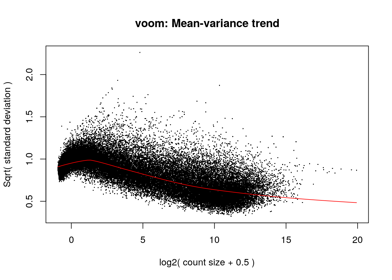


eb_results <- eBayes(lmFit(vGene))

de_results <- topTable(
    eb_results,
    coef = 2,
    number = nrow(rse_gene_SRP045638),
    sort.by = "none"
)
dim(de_results)
#> [1] 46929    16
head(de_results)
#>                    source type bp_length phase           gene_id                          gene_type gene_name level
#> ENSG00000223972.5  HAVANA gene      1735    NA ENSG00000223972.5 transcribed_unprocessed_pseudogene   DDX11L1     2
#> ENSG00000278267.1 ENSEMBL gene        68    NA ENSG00000278267.1                              miRNA MIR6859-1     3
#> ENSG00000227232.5  HAVANA gene      1351    NA ENSG00000227232.5             unprocessed_pseudogene    WASH7P     2
#>                            havana_gene  tag      logFC   AveExpr         t      P.Value    adj.P.Val         B
#> ENSG00000223972.5 OTTHUMG00000000961.2 <NA> -0.4522185 -3.444164 -1.637034 1.064080e-01 1.348462e-01 -5.554484
#> ENSG00000278267.1                 <NA> <NA>  1.1158860 -1.311645  6.123756 5.743771e-08 2.105690e-07  7.763912
#> ENSG00000227232.5 OTTHUMG00000000958.1 <NA>  0.6860298  3.641131  5.644804 3.816951e-07 1.247133e-06  5.500784
#>  [ reached 'max' / getOption("max.print") -- omitted 3 rows ]

## Differentially expressed genes between pre and post natal with FDR < 5%
table(de_results$adj.P.Val < 0.05)
#> 
#> FALSE  TRUE 
#> 12851 34078

## We can now visualize the resulting differential expression results
plotMA(eb_results, coef = 2)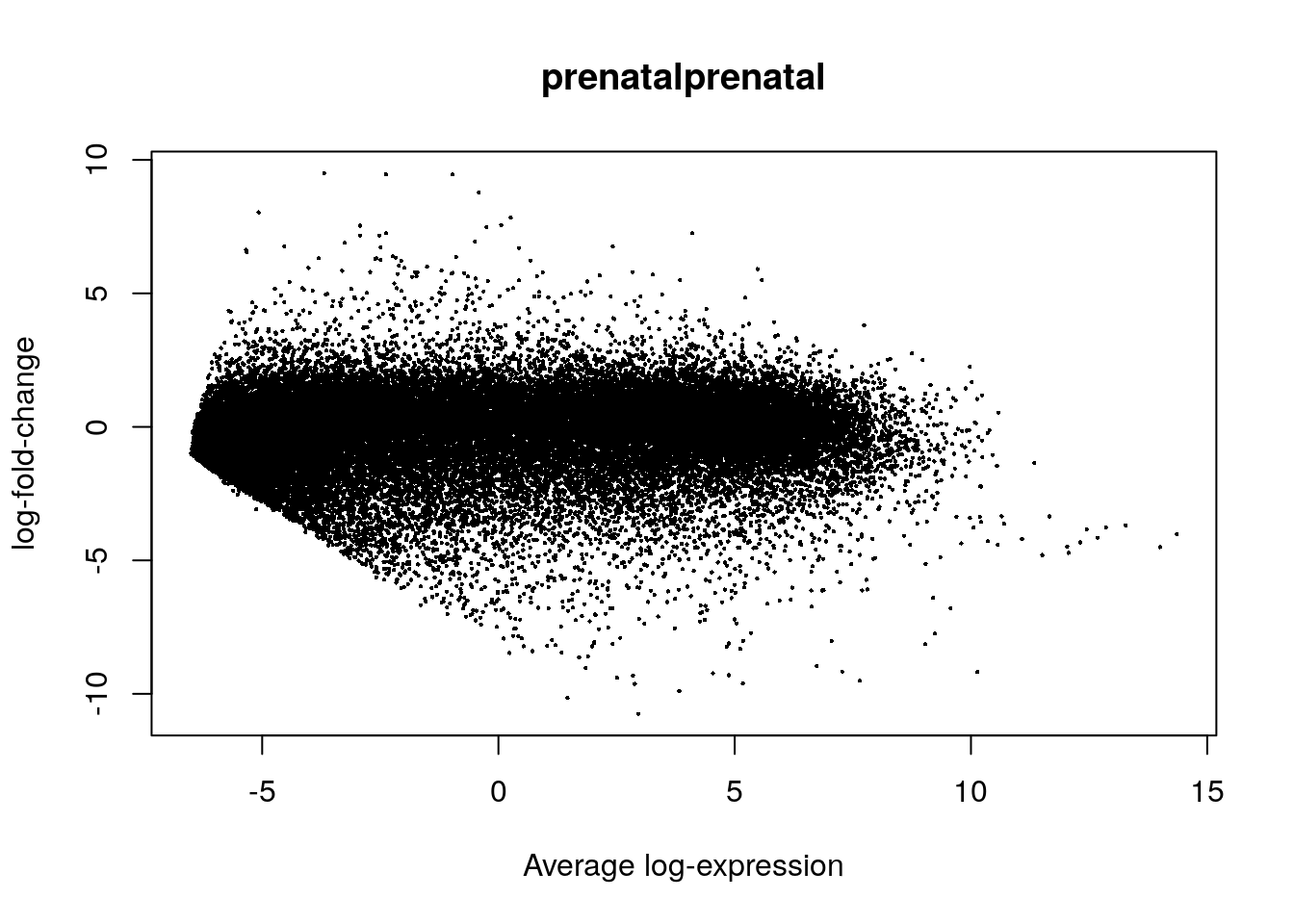


## We can also make a volcano plot
volcanoplot(eb_results, coef = 2, highlight = 3, names = de_results$gene_name)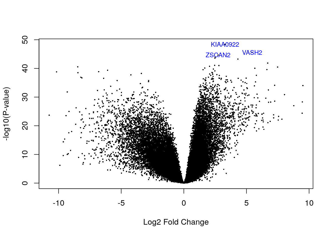

de_results[de_results$gene_name %in% c("ZSCAN2", "VASH2", "KIAA0922"), ]
#>                    source type bp_length phase            gene_id      gene_type gene_name level          havana_gene
#> ENSG00000143494.15 HAVANA gene      9086    NA ENSG00000143494.15 protein_coding     VASH2     2 OTTHUMG00000036925.5
#> ENSG00000176371.13 HAVANA gene      4878    NA ENSG00000176371.13 protein_coding    ZSCAN2     1 OTTHUMG00000074027.5
#> ENSG00000121210.15 HAVANA gene      6393    NA ENSG00000121210.15 protein_coding  KIAA0922     2 OTTHUMG00000153244.5
#>                     tag    logFC  AveExpr        t      P.Value    adj.P.Val         B
#> ENSG00000143494.15 <NA> 5.444271 1.876990 37.85216 2.561452e-46 6.010319e-42  95.10126
#> ENSG00000176371.13 <NA> 2.735639 2.751109 36.59344 2.137022e-45 3.342943e-41  92.99949
#> ENSG00000121210.15 <NA> 3.283050 2.945269 41.89725 4.235912e-49 1.987871e-44 101.31124

10.4 Visualizing DEGs

From vGene$E we can extract the normalized expression values that limma-voom computed. We can check the top 50 differentially expressed genes (DEGs) for example.

## Extract the normalized expression values from our limma-voom result
## from earlier
exprs_heatmap <- vGene$E[rank(de_results$adj.P.Val) <= 50, ]

## We can now build a table with information about our samples and
## then make the names a bit more friendly by making them easier to
## understand
df <- as.data.frame(colData(rse_gene_SRP045638)[, c("prenatal", "sra_attribute.RIN", "sra_attribute.sex")])
colnames(df) <- c("AgeGroup", "RIN", "Sex")

## Next, we can make a basic heatmap
library("pheatmap")
pheatmap(
    exprs_heatmap,
    cluster_rows = TRUE,
    cluster_cols = TRUE,
    show_rownames = FALSE,
    show_colnames = FALSE,
    annotation_col = df
)

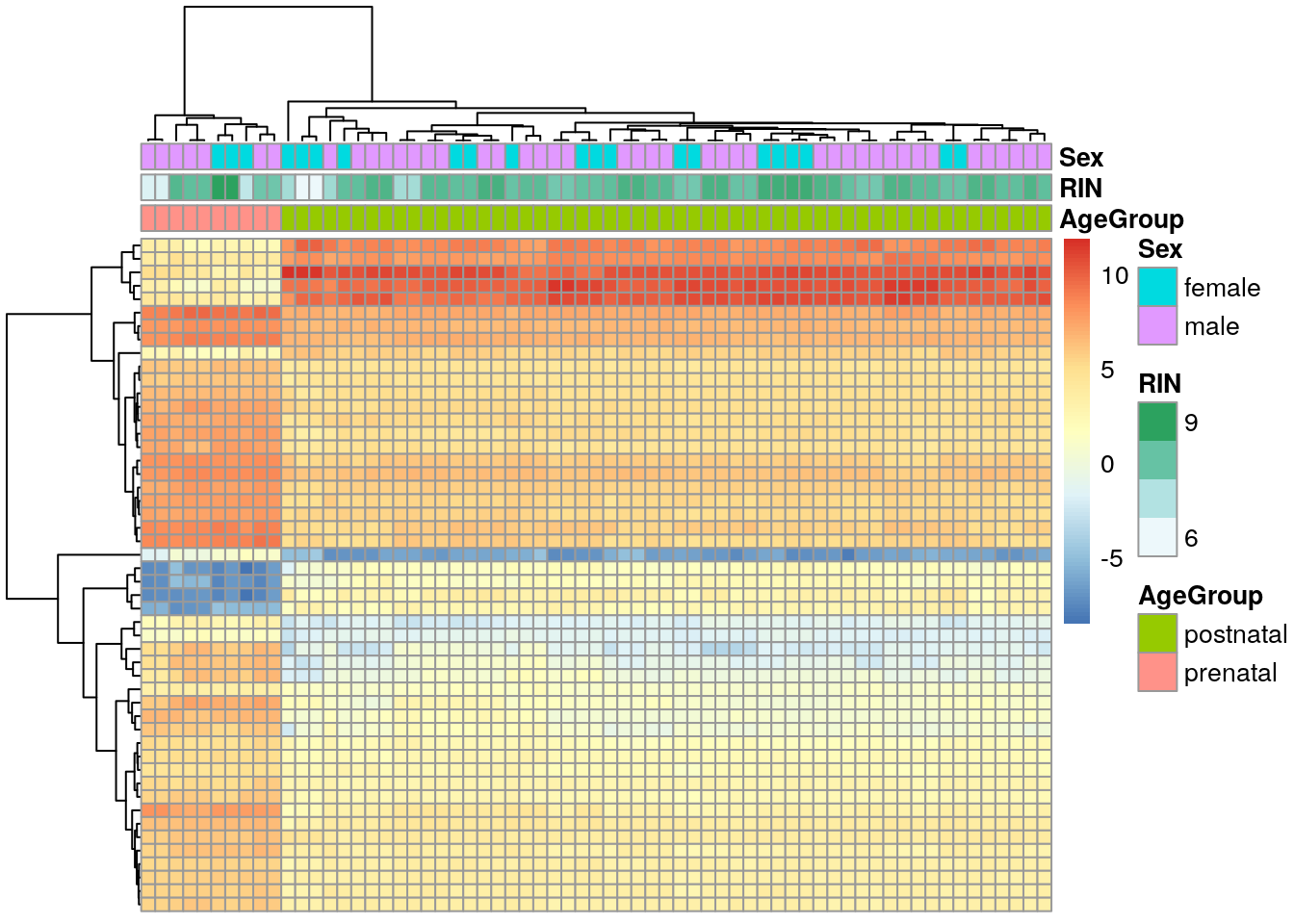
We’ll learn more about gene expression heatmaps tomorrow!

Overall, these DEG results are not as surprising since there is a huge difference between pre and post natal gene expression in the human DLPFC. We can see that more clearly with a MDS (multidimensional scaling) plot just like its described in the limma workflow. Tomas will teach you more about dimension reduction tomorrow.

## For nicer colors
library("RColorBrewer")

## Mapping age groups into colors
col.group <- df$AgeGroup
levels(col.group) <- brewer.pal(nlevels(col.group), "Set1")
#> Warning in brewer.pal(nlevels(col.group), "Set1"): minimal value for n is 3, returning requested palette with 3 different levels
col.group <- as.character(col.group)

## MDS by age groups
limma::plotMDS(vGene$E, labels = df$AgeGroup, col = col.group)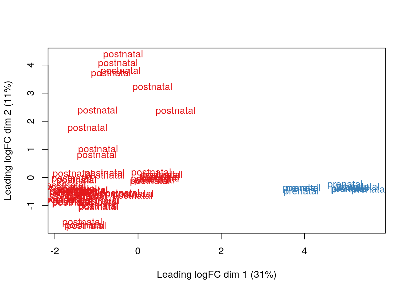


## Mapping Sex values into colors
col.sex <- df$Sex
levels(col.sex) <- brewer.pal(nlevels(col.sex), "Dark2")
#> Warning in brewer.pal(nlevels(col.sex), "Dark2"): minimal value for n is 3, returning requested palette with 3 different levels
col.sex <- as.character(col.sex)

## MDS by Sex
limma::plotMDS(vGene$E, labels = df$Sex, col = col.sex)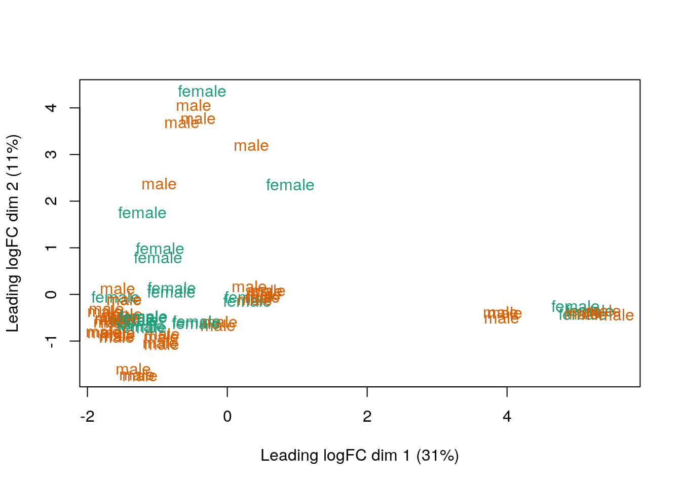

A lot of times, running the differential expression analysis is not the hard part. Building your model and having all the covariates you need can take much more work!

10.5 Community

Some edgeR and limma authors:

If you've ever been dazed by design matrices or confused by contrasts when performing gene expression analysis in limma, the new article by Charity Law is for you https://t.co/ZSMOA20tdm #bioconductor #rstats (1/2)
— Matt Ritchie (@mritchieau) December 15, 2020