18 Downloading public Visium spatial data and visualizing it with spatialLIBD

Instructor: Leo

18.1 Download data from 10x Genomics

We’ll run some code adapted from http://research.libd.org/spatialLIBD/articles/TenX_data_download.html (also available at https://bioconductor.org/packages/devel/data/experiment/vignettes/spatialLIBD/inst/doc/TenX_data_download.html). We’ll explore spatially resolved transcriptomics data from the Visium platform by 10x Genomics.

We’ll use BiocFileCache to keep the data in a local cache in case we want to run this example again and don’t want to re-download the data from the web.

## Download and save a local cache of the data provided by 10x Genomics
bfc <- BiocFileCache::BiocFileCache()
lymph.url <-
    paste0(
        "https://cf.10xgenomics.com/samples/spatial-exp/",
        "1.1.0/V1_Human_Lymph_Node/",
        c(
            "V1_Human_Lymph_Node_filtered_feature_bc_matrix.tar.gz",
            "V1_Human_Lymph_Node_spatial.tar.gz",
            "V1_Human_Lymph_Node_analysis.tar.gz"
        )
    )
lymph.data <- sapply(lymph.url, BiocFileCache::bfcrpath, x = bfc)
#> adding rname 'https://cf.10xgenomics.com/samples/spatial-exp/1.1.0/V1_Human_Lymph_Node/V1_Human_Lymph_Node_filtered_feature_bc_matrix.tar.gz'
#> adding rname 'https://cf.10xgenomics.com/samples/spatial-exp/1.1.0/V1_Human_Lymph_Node/V1_Human_Lymph_Node_spatial.tar.gz'
#> adding rname 'https://cf.10xgenomics.com/samples/spatial-exp/1.1.0/V1_Human_Lymph_Node/V1_Human_Lymph_Node_analysis.tar.gz'

10x Genomics provides the files in compressed tarballs (.tar.gz file extension). Which is why we’ll need to use utils::untar() to decompress the files. This will create new directories and we will use list.files() to see what files these directories contain.

## Extract the files to a temporary location
## (they'll be deleted once you close your R session)
xx <- sapply(lymph.data, utils::untar, exdir = file.path(tempdir(), "outs"))
## The names are the URLs, which are long and thus too wide to be shown here,
## so we shorten them to only show the file name prior to displaying the
## utils::untar() output status
names(xx) <- basename(names(xx))
xx
#> V1_Human_Lymph_Node_filtered_feature_bc_matrix.tar.gz.BFC4                    V1_Human_Lymph_Node_spatial.tar.gz.BFC5 
#>                                                          0                                                          0 
#>                   V1_Human_Lymph_Node_analysis.tar.gz.BFC6 
#>                                                          0

## List the files we downloaded and extracted
## These files are typically SpaceRanger outputs
lymph.dirs <- file.path(
    tempdir(), "outs",
    c("filtered_feature_bc_matrix", "spatial", "raw_feature_bc_matrix", "analysis")
)
list.files(lymph.dirs)
#>  [1] "aligned_fiducials.jpg"     "barcodes.tsv.gz"           "clustering"                "detected_tissue_image.jpg"
#>  [5] "diffexp"                   "features.tsv.gz"           "matrix.mtx.gz"             "pca"                      
#>  [9] "scalefactors_json.json"    "tissue_hires_image.png"    "tissue_lowres_image.png"   "tissue_positions_list.csv"
#> [13] "tsne"                      "umap"

18.2 Add gene annotation information

These files do not include much information about the genes, such as their chromosomes, coordinates, and other gene annotation information. We thus recommend that you read in this information from a gene annotation file: typically a gtf file. For a real case scenario, you’ll mostly likely have access to the GTF file provided by 10x Genomics. However, we cannot download that file without downloading other files for this example.

18.2.1 From 10x

Depending on the version of spaceranger you used, you might have used different GTF files 10x Genomics has made available at https://support.10xgenomics.com/single-cell-gene-expression/software/downloads/latest and described at https://support.10xgenomics.com/single-cell-gene-expression/software/release-notes/build. These files are too big though and we won’t download them in this example. For instance, References - 2020-A (July 7, 2020) for Human reference (GRCh38) is 11 GB in size and contains files we do not need here. If you did have the file locally, we would just need the path to this GTF file later.

For example, in our computing cluster this GTF file is located at the following path and is 1.4 GB in size:

$ cd /dcs04/lieber/lcolladotor/annotationFiles_LIBD001/10x/refdata-gex-GRCh38-2020-A
$ du -sh --apparent-size genes/genes.gtf
1.4G    genes/genes.gtf

18.2.2 From Gencode

In the absence of the GTF file used by 10x Genomics, we’ll use the GTF file from Gencode v32 which we can download and that is much smaller. That’s because the build notes from References - 2020-A (July 7, 2020) and Human reference, GRCh38 (GENCODE v32/Ensembl 98) at https://support.10xgenomics.com/single-cell-gene-expression/software/release-notes/build#GRCh38_2020A show that 10x Genomics used Gencode v32. They also used Ensembl version 98 which is why a few genes we have in our object are going to be missing. Let’s download this GTF file.

## Download the Gencode v32 GTF file and cache it
gtf_cache <- BiocFileCache::bfcrpath(
    bfc,
    paste0(
        "ftp://ftp.ebi.ac.uk/pub/databases/gencode/Gencode_human/",
        "release_32/gencode.v32.annotation.gtf.gz"
    )
)
#> adding rname 'ftp://ftp.ebi.ac.uk/pub/databases/gencode/Gencode_human/release_32/gencode.v32.annotation.gtf.gz'

## Show the GTF cache location
gtf_cache
#>                                                                            BFC7 
#> "/github/home/.cache/R/BiocFileCache/48f6246c5ff_gencode.v32.annotation.gtf.gz"

18.3 Wrapper functions for reading the data

To facilitate reading in the data and preparing it to visualize it interactively using spatialLIBD::run_app(), we implemented read10xVisiumWrapper() which expands SpatialExperiment::read10xVisium() and performs the steps described in more detail at http://research.libd.org/spatialLIBD/articles/TenX_data_download.html. In this example, we’ll load all four images created by SpaceRanger: lowres, hires, detected, and aligned. That way we can toggle between them on the web application.

## Import the data as a SpatialExperiment object using wrapper functions
## provided by spatialLIBD
library("spatialLIBD")
spe_wrapper <- read10xVisiumWrapper(
    samples = file.path(tempdir(), "outs"),
    sample_id = "lymph",
    type = "sparse", data = "filtered",
    images = c("lowres", "hires", "detected", "aligned"), load = TRUE,
    reference_gtf = gtf_cache
)
#> 2023-07-11 23:15:06.689031 SpatialExperiment::read10xVisium: reading basic data from SpaceRanger
#> 2023-07-11 23:15:29.987538 read10xVisiumAnalysis: reading analysis output from SpaceRanger
#> 2023-07-11 23:15:30.158091 add10xVisiumAnalysis: adding analysis output from SpaceRanger
#> 2023-07-11 23:15:30.633049 rtracklayer::import: reading the reference GTF file
#> 2023-07-11 23:16:16.209258 adding gene information to the SPE object
#> Warning: Gene IDs did not match. This typically happens when you are not using the same GTF file as the one that was
#> used by SpaceRanger. For example, one file uses GENCODE IDs and the other one ENSEMBL IDs. read10xVisiumWrapper() will
#> try to convert them to ENSEMBL IDs.
#> Warning: Dropping 29 out of 36601 genes for which we don't have information on the reference GTF file. This typically
#> happens when you are not using the same GTF file as the one that was used by SpaceRanger.
#> 2023-07-11 23:16:16.726447 adding information used by spatialLIBD

## Explore the resulting SpatialExperiment object
spe_wrapper
#> class: SpatialExperiment 
#> dim: 36572 4035 
#> metadata(0):
#> assays(1): counts
#> rownames(36572): ENSG00000243485.5 ENSG00000237613.2 ... ENSG00000198695.2 ENSG00000198727.2
#> rowData names(6): source type ... gene_type gene_search
#> colnames(4035): AAACAAGTATCTCCCA-1 AAACAATCTACTAGCA-1 ... TTGTTTGTATTACACG-1 TTGTTTGTGTAAATTC-1
#> colData names(20): sample_id in_tissue ... expr_chrM_ratio ManualAnnotation
#> reducedDimNames(3): 10x_pca 10x_tsne 10x_umap
#> mainExpName: NULL
#> altExpNames(0):
#> spatialCoords names(2) : pxl_col_in_fullres pxl_row_in_fullres
#> imgData names(4): sample_id image_id data scaleFactor

## Size of the data
lobstr::obj_size(spe_wrapper)
#> 410.19 MB

## Run our shiny app
if (interactive()) {
    vars <- colnames(colData(spe_wrapper))

    run_app(
        spe_wrapper,
        sce_layer = NULL,
        modeling_results = NULL,
        sig_genes = NULL,
        title = "spatialLIBD: human lymph node by 10x Genomics (made with wrapper)",
        spe_discrete_vars = c(vars[grep("10x_", vars)], "ManualAnnotation"),
        spe_continuous_vars = c("sum_umi", "sum_gene", "expr_chrM", "expr_chrM_ratio"),
        default_cluster = "10x_graphclust"
    )
}

The result should look pretty much like https://libd.shinyapps.io/spatialLIBD_Human_Lymph_Node_10x/.

The apps showcased above are linked to and described at http://research.libd.org/spatialDLPFC/#interactive-websites. This video was part of Nicholas J. Eagles recent LIBD seminar presentation.

Congrats Nick for successfully completing your 1st🥇 @LieberInstitute seminar 🙌🏽

Nick presented #spatialDLPFC spot deconvolution results @10xGenomics #snRNAseq #Visium #VisiumSPG

🛝 https://t.co/2wMLSkTLyW

Interact with the data https://t.co/ya4oyiMVsN https://t.co/cTdGNswysy pic.twitter.com/Ggmnnmj2nA
— 🇲🇽 Leonardo Collado-Torres (@lcolladotor) June 27, 2023

18.4 Visualize spatial plots

Now that we have explored the spatially resolved transcriptomics data with the spatialLIBD::run_app() shiny website, lets make some plots ourselves.

Check out the documentation for these two functions:

spatialLIBD::vis_gene() http://research.libd.org/spatialLIBD/reference/vis_gene.html for continuous variables, including gene expression values
spatialLIBD::vis_clus() http://research.libd.org/spatialLIBD/reference/vis_clus.html for discrete variables

18.5 Exercise

Exercise 1:

Plot a discrete variable of your choice with and without the histology image on the background.
- For example, visualize the k-means with \(k = 10\) clustering results computed by SpaceRanger.
Use custom colors of your choice. See https://emilhvitfeldt.github.io/r-color-palettes/discrete.html to choose a color palette.
- For example, use the Polychrome::palette36() colors.

Solution 1: The function for plotting discrete variables is spatialLIBD::vis_clus() which is documented at http://research.libd.org/spatialLIBD/reference/vis_clus.html. After reading the documentation website for this function, we are ready to write the code to solve our exercise problem.

## Basic spatial graph visualizing a discrete variable that we provided to
## the argument "clustervar". Here we chose to visualize
## "10x_kmeans_10_clusters" which contains the clustering results from the
## K-means algorithm when k = 10.
## We are plotting the one sample we have called "lymph". This is the same
## name we chose earlier when we ran spatialLIBD::read10xVisiumWrapper().
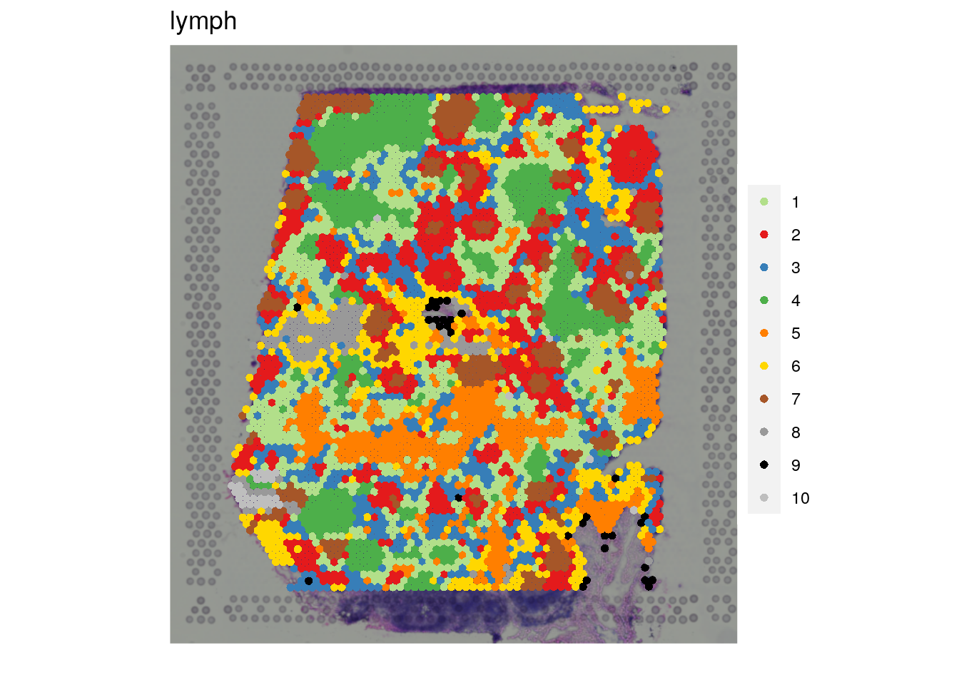
vis_clus(
    spe = spe_wrapper,
    sampleid = "lymph",
    clustervar = "10x_kmeans_10_clusters"
)


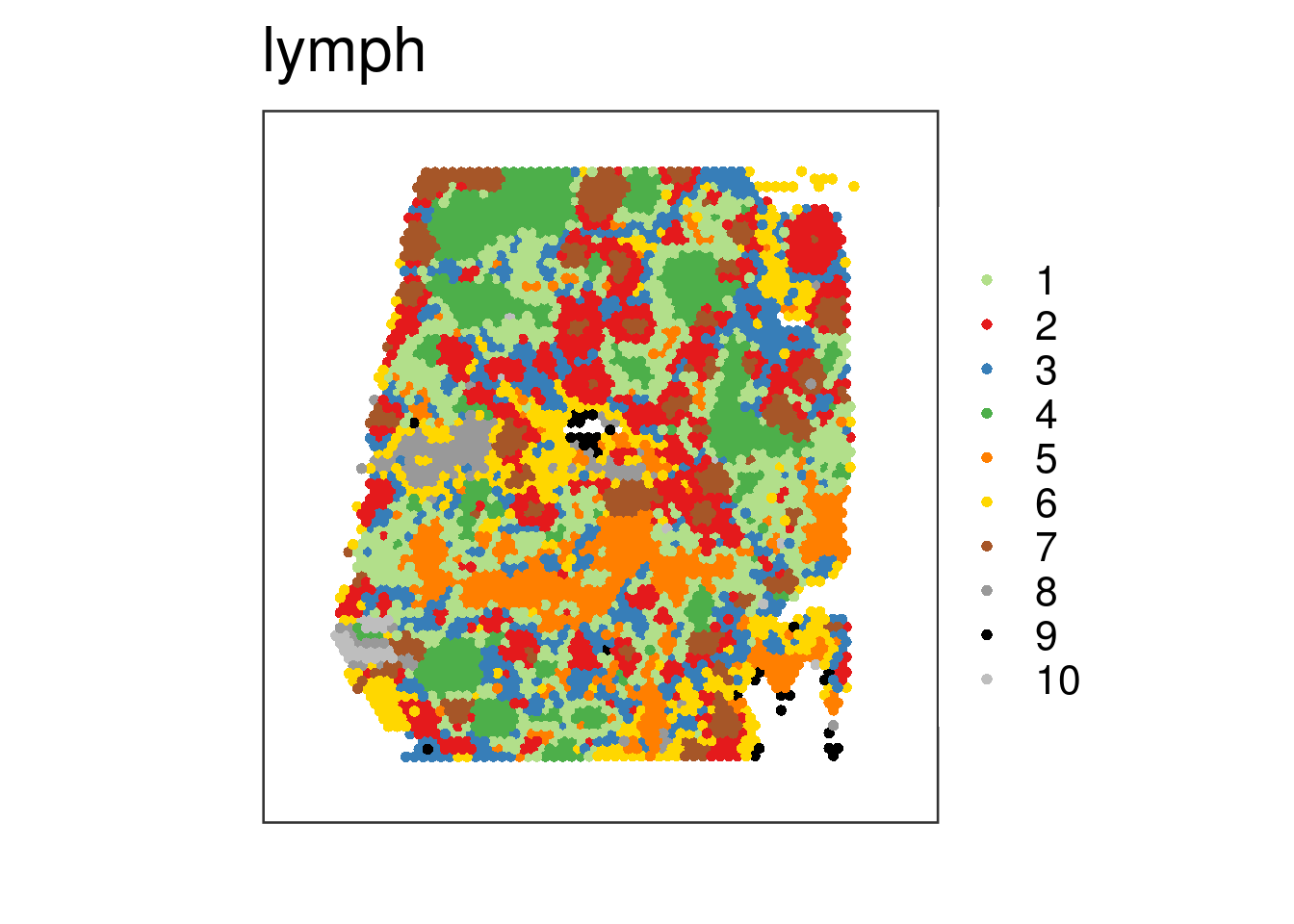
## Next we ignore the histology image and stop plotting it by setting
## "spatial = FALSE"
vis_clus(
    spe = spe_wrapper,
    sampleid = "lymph",
    clustervar = "10x_kmeans_10_clusters",
    spatial = FALSE
)


## Finally, we use the "colors" argument to specify our own colors. We use
## the general setNames() R function to create a named vector that has as
## values the colors and as names the same names we have for our "clustervar".
vis_clus(
    spe = spe_wrapper,
    sampleid = "lymph",
    clustervar = "10x_kmeans_10_clusters",
    spatial = FALSE,
    colors = setNames(Polychrome::palette36.colors(10), 1:10)
)


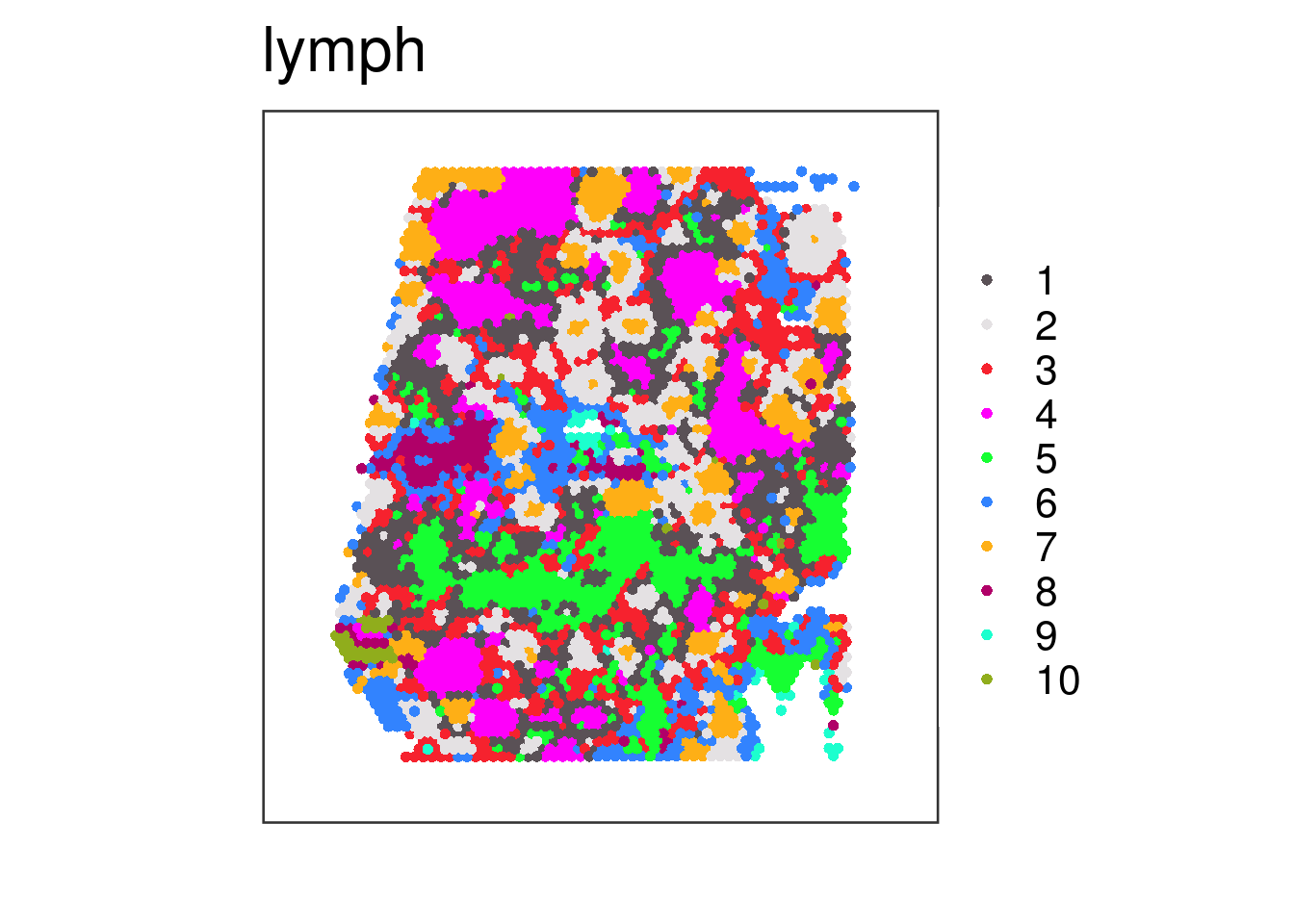
## Here we can see the vector we provided as input to "colors":
setNames(Polychrome::palette36.colors(10), 1:10)
#>         1         2         3         4         5         6         7         8         9        10 
#> "#5A5156" "#E4E1E3" "#F6222E" "#FE00FA" "#16FF32" "#3283FE" "#FEAF16" "#B00068" "#1CFFCE" "#90AD1C"