2 Interactive SummarizedExperiment visualizations
Instructor: Melissa Mayén Quiroz
How can you make plots from “SummarizedExperiment” objects without having to write any code?
The answer is with “iSEE”
- http://bioconductor.org/packages/iSEE
- http://bioconductor.org/packages/release/bioc/vignettes/iSEE/inst/doc/basic.html
iSEE is a Bioconductor package that provides an interactive Shiny-based graphical user interface for exploring data stored in SummarizedExperiment objects (Rue-Albrecht et al. 2018).
2.1 Classes for iSEE
SummarizedExperiment (SE) and SingleCellExperiment (SCE) are classes in R. Classes serve as templates for creating objects that contain data and methods for manipulating those data.
2.1.1 SummarizedExperiment class
Assay Data: The primary data matrix containing quantitative measurements, such as gene expression values or read counts. Rows represent features (e.g., genes, transcripts) and columns represent samples (e.g., experimental conditions, individuals).
Row Metadata (
rowData): Additional information about the features in the assay data. This can include annotations, identifiers, genomic coordinates, and other relevant information.Column Metadata (
colData): Additional information about the samples in the assay data. This can include sample annotations, experimental conditions, treatment groups, and other relevant information.metadata: Additional information about the experiment.
2.1.2 SingleCellExperiment
This object is specifically designed to store and analyze single-cell RNA sequencing (scRNA-seq) data. It extends the SummarizedExperiment class to include specialized features for single-cell data, such as cell identifiers, dimensionality reduction results, and methods for quality control and normalization.
Assay Data: The primary data matrix containing gene expression values or other measurements. Rows represent genes and columns represent cells.
colData(Column Metadata): Additional information about each cell, such as cell type, experimental condition, or any other relevant metadata.rowData(Row Metadata): Additional information about each gene, such as gene symbols, genomic coordinates, or functional annotations.reducedDims: Dimensionality reduction results, such as “principal component analysis” (PCA), “t-distributed stochastic neighbor embedding” (t-SNE), and “Uniform Manifold Approximation and Projection” (UMAP), used for visualizing and clustering cells.altExpNamesandaltExps: Names of alternative experiments (such as spike-in control genes used for normalization) and alternative experiment counts matrices.metadata: Additional metadata about the experiment.
2.1.3 SpatialExperiment
This object extends the SingleCellExperiment class and is designed to store and analyze spatially-resolved transcriptomics data. Spatial transcriptomics combines gene expression data with spatial information, providing insights into the spatial organization of tissues.
Assay Data: The primary data matrix containing gene expression values or other measurements. Rows represent genes and columns represent spatial spots or pixels.
colData(Column Metadata): Additional information about each spatial spot or pixel, such as spatial coordinates, tissue section, or any other relevant metadata.rowData(Row Metadata): Additional information about each gene, such as gene symbols, genomic coordinates, or functional annotations.spatialCoords: A matrix or data frame containing the spatial coordinates (e.g., x and y coordinates) of each spot or pixel, which is crucial for spatial analyses and visualization.imgData: Links to image data associated with the spatial transcriptomics experiment, such as histology images or microscopy images, which provide the spatial context for the transcriptomics data.reducedDims: Dimensionality reduction results for visualizing and clustering spatial spots or pixels, similar to the SingleCellExperiment class.metadata: Additional metadata about the experiment.
2.2 Getting Started with iSEE
Adapted from The iSEE User’s Guide
- Installation (R version “4.4”). In this case, the package is already installed so we just need to load it.
# if (!require("BiocManager", quietly = TRUE))
#     install.packages("BiocManager")
#
# BiocManager::install("iSEE")

packageVersion("iSEE")
#> [1] '2.16.0'- Documentation
- Use (simple launch):
If you have a SummarizedExperiment object (se) or an instance of a subclass, like a SingleCellExperiment object (sce), you can launch an iSEE app by running:
2.3 Description of the user interface
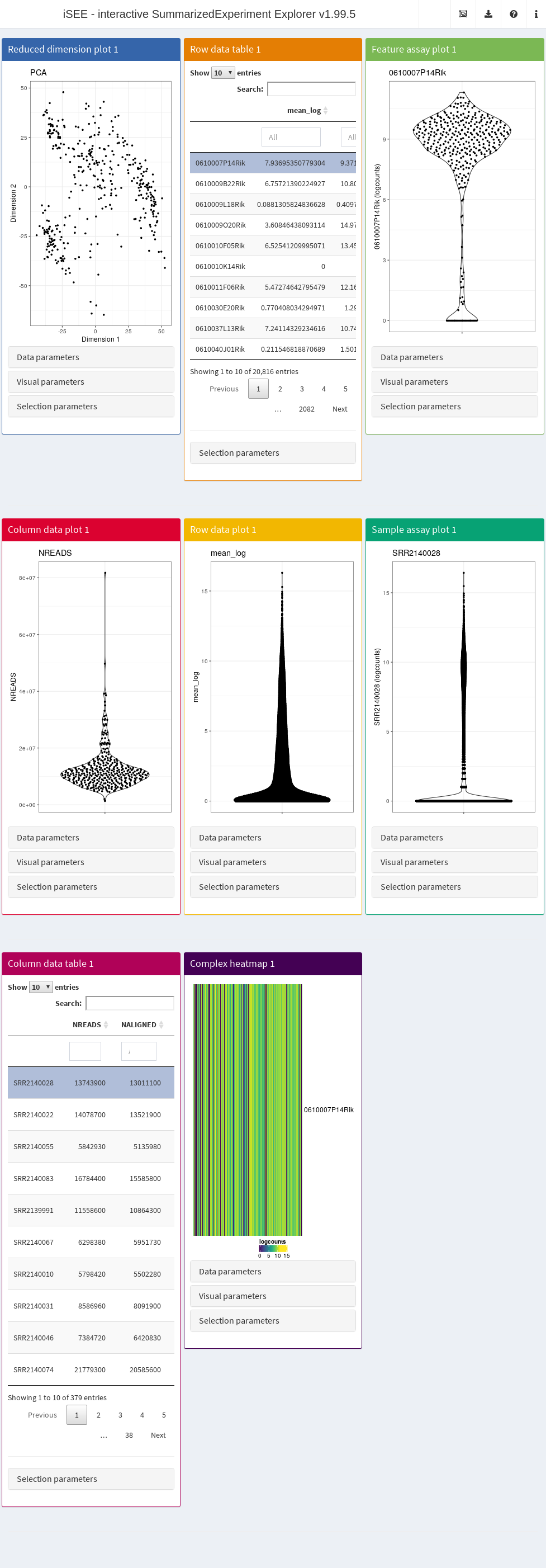
By default, the app starts with a dashboard that contains one panel or table of each type. By opening the collapsible panels named “Data parameters”, “Visual parameters”, and “Selection parameters” under each plot, we can control the content and appearance of each panel.
Introductory tour:
In the upper right corner there is a question mark icon ❓. Clicking it and then on the hand button you can have an introductory tour. During this tour, you will be taken through the different components of the iSEE user interface and learn the basic usage mechanisms by doing small actions guided by the tutorial: the highlighted elements will be responding to your actions, while the rest of the UI will be shaded.
2.3.1 Header
The layout of the iSEE user interface uses the shinydashboard package. The dashboard header contains four dropdown menus.
- The “Organization” menu, which is identified by an icon displaying multiple windows
- “Export” dropdown menu, which is identified by a download icon
- The “Documentation” dropdown menu which is identified by a question mark icon ❓
- The “Additional Information” dropdown menu which is identified by the information icon ℹ️
2.3.2 Panel types
The main element in the body of iSEE is the combination of panels, generated (and optionally linked to one another) according to your actions. There are currently eight standard panel types that can be generated with iSEE:
- Reduced dimension plot
- Column data table
- Column data plot
- Feature assay plot
- Row data table
- Row data plot
- Sample assay plot
- Complex heatmap
In addition, custom panel types can be defined.
2.3.3 Parameter sets
For each standard plot panel, three different sets of parameters will be available in collapsible boxes:
“Data parameters”, to control parameters specific to each type of plot.
“Visual parameters”, to specify parameter s that will determine the aspect of the plot, in terms of coloring, point features, and more (e.g., legend placement, font size).
“Selection parameters” to control the incoming point selection and link relationships to other plots.
2.3.4 Reduced dimension plots
If a SingleCellExperiment object is supplied to the iSEE::iSEE() function, reduced dimension results are extracted from the reducedDim slot.
Examples include low-dimensional embeddings from principal components analysis (PCA) or t-distributed stochastic neighbour embedding (t-SNE). These results are used to construct a two-dimensional Reduced dimension plot where each point is a sample, to facilitate efficient exploration of high-dimensional datasets. The “Data parameters” control the reducedDim slot to be displayed, as well as the two dimensions to plot against each other.
Note that this built in panel does not compute reduced dimension embeddings; they must be precomputed and available in the object provided to the iSEE() function. Nevertheless, custom panels - such as the iSEE DynamicReducedDimensionPlot can be developed and used to enable such features.
2.3.5 Column data plots
A Column data plot visualizes sample metadata contained in column metadata. Different fields can be used for the x- and y-axes by selecting appropriate values in the “Data parameters” box. This plot can assume various forms, depending on the nature of the data on the x- and y-axes:
If the y-axis is continuous and the x-axis is categorical, violin plots are generated (grouped by the x-axis factor).
If the y-axis is categorical and the x-axis is continuous, horizontal violin plots are generated (grouped by the y-axis factor).
If both axes are continuous, a scatter plot is generated. This enables the use of contours that are overlaid on top of the plot, check the “Other” box to see the available options.
If both axes are categorical, a plot of squares (Hinton plot) is generated where the area of each square is proportional to the number of samples within each combination of factor levels.
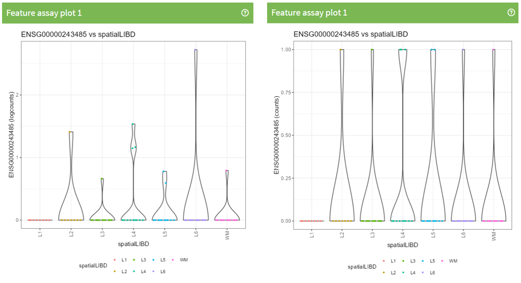
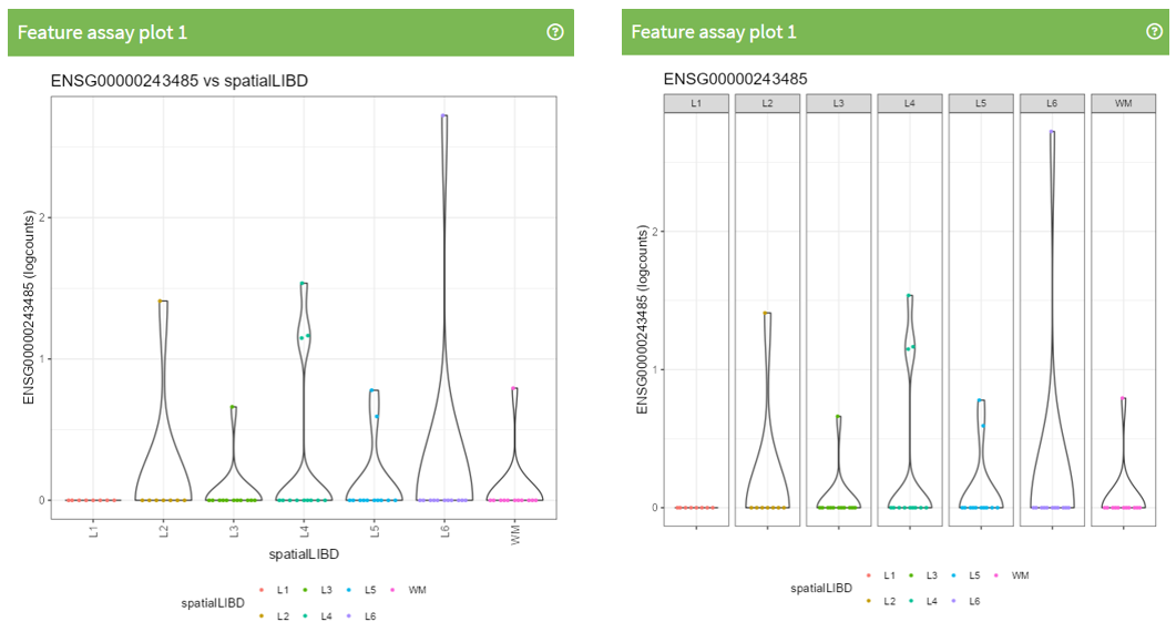
2.3.6 Feature assay plots
A Feature assay plot visualizes the assayed values (e.g., gene expression) for a particular feature (e.g., gene) across the samples on the y-axis. This usually results in a (grouped) violin plot, if the x-axis is set to “None” or a categorical variable; or a scatter plot, if the x-axis is another continuous variable.
Gene selection for the y-axis can be achieved by using a linked row data table in another panel. Clicking on a row in the table automatically changes the assayed values plotted on the y-axis. Alternatively, the row name can be directly entered as text that corresponds to an entry of rownames(se). (This is not effective if se does not contain row names.)
2.3.7 Row data plots
A Row data plot allows the visualization of information stored in the rowData slot of a “SummarizedExperiment” object. Its behavior mirrors the implementation for the Column data plot, and correspondingly this plot can assume various forms depending on whether the data are categorical or continuous.
2.3.8 Sample assay plots
A Sample assay plot visualizes the assayed values (e.g., gene expression) for a particular sample (e.g., cell) across the features on the y-axis.
This usually results in a (grouped) violin plot, if the x-axis is set to “None” or a categorical variable (e.g., gene biotype); or a scatter plot, if the x-axis is another continuous variable.
Notably, the x-axis covariate can also be set to:
A discrete row data covariates (e.g., gene biotype), to stratify the distribution of assayed values
A continuous row data covariate (e.g., count of cells expressing each gene)
Another sample, to visualize and compare the assayed values in any two samples.
2.3.9 Row data tables
A Row data table contains the values of the rowData slot. If none are available, a column named Present is added and set to TRUE for all features, to avoid issues with DT::datatable() and an empty DataFrame.
Typically, these tables are used to link to other plots to determine the features to use for plotting or coloring.
2.3.10 Column data tables
A Column data table contains the values of the colData slot. Its behavior mirrors the implementation for the Row data table. Correspondingly, if none are available, a column named Present is added and set to TRUE for all samples.
Typically, these tables are used to link to other plots to determine the samples to use for plotting or coloring.
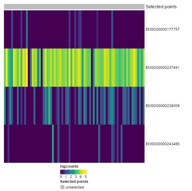
2.3.11 Heat maps
Heat map panels provide a compact overview of the data for multiple features in the form of color-coded matrices. These correspond to the assays stored in the SCE/SE object, where features (e.g., genes) are the rows and samples are the columns.
User can select features (rows) to display from the selectize widget (which supports autocompletion), or also via other panels, like row data plots or row data tables. In addition, users can rapidly import custom lists of feature names using a modal popup that provides an Ace editor where they can directly type of paste feature names, and a file upload button that accepts text files containing one feature name per line. Users should remember to click the “Apply” button before closing the modal, to update the heat map with the new list of features.
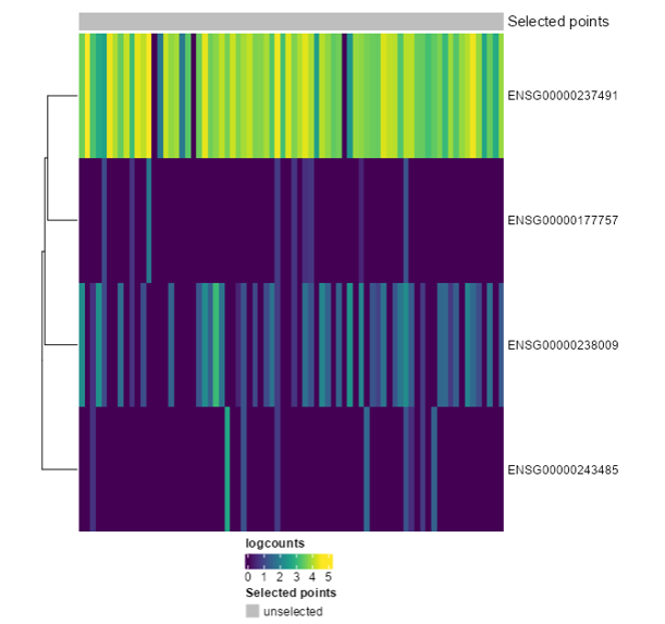
The “Suggest feature order” button clusters the rows, and also rearranges the elements in the selectize according to the clustering.
It is also possible to choose which assay type is displayed ("logcounts" being the default choice, if available).
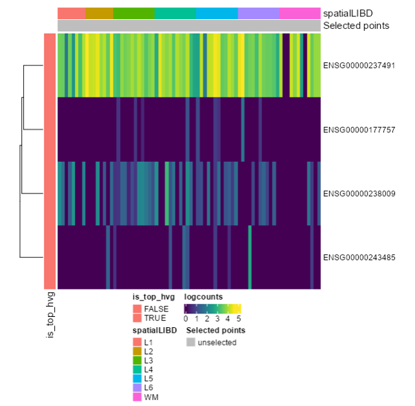
Samples in the heat map can also be annotated, simply by selecting relevant column metadata.
A zooming functionality is also available, restricted to the y-axis (i.e., allowing closer inspection on the individual features included).
2.3.12 Description of iSEE functionality
2.3.12.1 Coloring plots by sample attributes
2.3.12.1.1 Column-based plots
Column-based plots are:
reduced dimension
feature assay
column data plots
Where each data point represents a sample. Here, data points can be colored in different ways:
The default is no color scheme (“None” in the radio button).
Any column of colData(se) can be used. The plot automatically adjusts the scale to use based on whether the chosen column is continuous or categorical.
The assay values of a particular feature in each sample can be used. The feature can be chosen either via a linked row table or selectize input (as described for the Feature assay plot panel). Users can also specify the assays from which values are extracted.
The identity of a particular sample can be used, which will be highlighted on the plot in a user-specified color. The sample can be chosen either via a linked column table or via a selectize input.
2.3.12.1.2 Row-based plots
For row-based plots (i.e., the sample assay and row data plots), each data point represents a feature. Like the column-based plots, data points can be colored by:
“None”, yielding data points of fixed color.
Any column of
rowData(se).The identity of a particular feature, which is highlighted in the user-specified color.
Assay values for a particular sample.
2.3.12.2 Controlling point aesthetics
Data points can be set to different shapes according to categorical factors in colData(se) (for column-based plots) or rowData(se) (for row-based plots). This is achieved by checking the “Shape” box to reveal the shape-setting options. The size and opacity of the data points can be modified via the options available by checking the “Point” box. This may be useful for aesthetically pleasing visualizations when the number of points is very large or small.
2.3.12.3 Faceting
Each point-based plot can be split into multiple facets using the options in the “Facet” checkbox. Users can facet by row and/or column, using categorical factors in colData(se) (for column-based plots) or rowData(se) (for row-based plots). This provides a convenient way to stratify points in a single plot by multiple factors of interest. Note that point selection can only occur within a single facet at a time; points cannot be selected across facets.
2.4 Let’s practice!
2.4.1 Setting up the data
- We’ll download a
SingleCellExperimentobject, which is similar toSummarizedExperimentas it extends it.
## Lets get some data using spatialLIBD
sce_layer <- spatialLIBD::fetch_data("sce_layer")
#> adding rname 'https://www.dropbox.com/s/bg8xwysh2vnjwvg/Human_DLPFC_Visium_processedData_sce_scran_sce_layer_spatialLIBD.Rdata?dl=1'
#> 2024-06-11 20:00:07.007194 loading file /github/home/.cache/R/BiocFileCache/3c175dc2d1f_Human_DLPFC_Visium_processedData_sce_scran_sce_layer_spatialLIBD.Rdata%3Fdl%3D1
sce_layer
#> class: SingleCellExperiment
#> dim: 22331 76
#> metadata(0):
#> assays(2): counts logcounts
#> rownames(22331): ENSG00000243485 ENSG00000238009 ... ENSG00000278384 ENSG00000271254
#> rowData names(10): source type ... is_top_hvg is_top_hvg_sce_layer
#> colnames(76): 151507_Layer1 151507_Layer2 ... 151676_Layer6 151676_WM
#> colData names(13): sample_name layer_guess ... layer_guess_reordered_short spatialLIBD
#> reducedDimNames(6): PCA TSNE_perplexity5 ... UMAP_neighbors15 PCAsub
#> mainExpName: NULL
#> altExpNames(0):NOTE: if you run into this error:
Error in `BiocFileCache::bfcrpath()`:
! not all 'rnames' found or unique.
Backtrace:
 1. spatialLIBD::fetch_data("sce_layer")
 3. BiocFileCache::bfcrpath(bfc, url)
check the output of
If it’s version 8.6.0, you likely need to upgrade to version 8.8.0. For macOS users, you can do this via Homebrew with
then install curl from source with:
Sys.setenv(PKG_CONFIG_PATH = "/opt/homebrew/opt/curl/lib/pkgconfig")
install.packages("curl", type = "source")
For all the gory details, check https://github.com/curl/curl/issues/13725, https://github.com/Bioconductor/BiocFileCache/issues/48, and related issues.
As a workaround, you could also run this:
tmp_sce_layer <- tempfile("sce_layer.RData")
download.file(
    "https://www.dropbox.com/s/bg8xwysh2vnjwvg/Human_DLPFC_Visium_processedData_sce_scran_sce_layer_spatialLIBD.Rdata?dl=1",
    tmp_sce_layer,
    mode = "wb"
)
load(tmp_sce_layer, verbose = TRUE)
#> Loading objects:
#>   sce_layer
sce_layer
#> class: SingleCellExperiment
#> dim: 22331 76
#> metadata(0):
#> assays(2): counts logcounts
#> rownames(22331): ENSG00000243485 ENSG00000238009 ... ENSG00000278384 ENSG00000271254
#> rowData names(10): source type ... is_top_hvg is_top_hvg_sce_layer
#> colnames(76): 151507_Layer1 151507_Layer2 ... 151676_Layer6 151676_WM
#> colData names(12): sample_name layer_guess ... layer_guess_reordered layer_guess_reordered_short
#> reducedDimNames(6): PCA TSNE_perplexity5 ... UMAP_neighbors15 PCAsub
#> mainExpName: NULL
#> altExpNames(0):2.4.2 Explore the Data
Now we can deploy iSEE() to explore the data.
Question 1: Which panel Type is displaying the following plot?
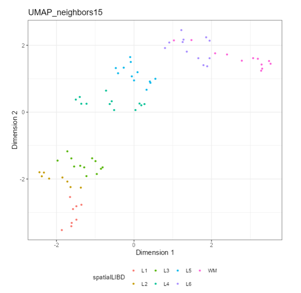
Exercise 1: Recreate the following plot.
Question 2: What is different between this 2 plots?
Exercise 2: Recreate the following plot.
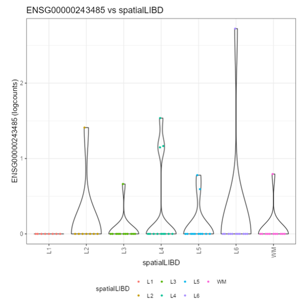
Question 3: What is different between this 2 plots?
Exercise 3: Recreate the following plot
Ensembl IDs: ENSG00000177757 ENSG00000237491 ENSG00000238009 ENSG00000243485
Exercise 4: Recreate the following plot. What would you change from the last one?
Ensembl IDs: ENSG00000177757 ENSG00000237491 ENSG00000238009 ENSG00000243485
Exercise 5: Recreate the following plot. What would you change from the last one?
Ensembl IDs: ENSG00000177757 ENSG00000237491 ENSG00000238009 ENSG00000243485
Exercise 6: Download only the last plot (Final HeatMap)
Exercise 7: Extract the R code only for the last plot (Final HeatMap)
2.5 Introduction to Advanced iSEE Features
Adapted from the GitHub Issue: https://github.com/iSEE/iSEE/issues/650
Beyond its basic functionalities, iSEE offers advanced features that allow users to perform complex data manipulations interactively. This includes the ability to subset and filter cells based on gene expression criteria.
To begin with, we will load the necessary libraries and dataset. In this case we will be using ReprocessedAllenData from the scRNAseq package, a dataset of 379 mouse brain cells from Tasic et al. (2016).
After loading the dataset, we normalize the counts and perform a PCA (Principal Component Analysis) to prepare the data for visualization.
library("scRNAseq")
library("scater")
library("iSEE")

# Load the dataset
sce <- ReprocessedAllenData(assays = "tophat_counts")

# Normalize counts and perform PCA
sce <- logNormCounts(sce, exprs_values = "tophat_counts")
sce <- runPCA(sce, ncomponents = 4)
2.5.1 Selecting Cells Based on a Single Gene Expression
To select cells based on the expression of a single gene using iSEE, we need to create an initial list of panels that will be displayed when we launch iSEE. The first panel in our list is a “FeatureAssayPlot”, which will show the expression levels of the gene “Serpine2”. By visualizing this plot, we can interactively select cells that express “Serpine2”.
To complement this, we add a “ReducedDimensionPlot” to our panel list. This plot will visualize the PCA and highlight the cells that we selected based on “Serpine2” expression. The linkage between these two panels allows us to see how the selected cells are distributed in the reduced dimensional space (PCA).
## Initial settings for a single gene expression
initial_single <- list(
    FeatureAssayPlot(Assay = "logcounts", YAxisFeatureName = "Serpine2"),
    ReducedDimensionPlot(Type = "PCA", ColorBy = "Column selection", ColumnSelectionSource = "FeatureAssayPlot1")
)

## Launch iSEE with the initial settings
if (interactive()) {
    iSEE(sce, initial = initial_single)
}
2.5.2 Using a Single Plot for Two Gene Co-Expression
To select cells based on the expression of two gene, we can use a single “FeatureAssayPlot” panel. In this setup, one gene is plotted on the x-axis and the other gene on the y-axis. This method allows us to directly visualize and select cells that express both genes simultaneously.
By adding a “ReducedDimensionPlot” to our initial panel list, we can again see how these selected cells are distributed in the PCA plot. This approach is simpler when dealing with only two genes and provides an intuitive way to explore co-expression patterns.
## Initial settings for 2 genes expression on the same "FeatureAssayPlot"
initial_combined <- list(
    FeatureAssayPlot(Assay = "logcounts", XAxis = "Feature name", XAxisFeatureName = "Serpine2", YAxisFeatureName = "Bcl6"),
    ReducedDimensionPlot(Type = "PCA", ColorBy = "Column selection", ColumnSelectionSource = "FeatureAssayPlot1")
)

## Launch iSEE with the initial settings
if (interactive()) {
    iSEE(sce, initial = initial_combined)
}
2.5.3 Selecting Cells Based on the Co-Expression of Two or more Genes
In situations where we want to select cells based on the expression of two or more genes, we need to chain multiple “FeatureAssayPlot” panels together. For instance, if we are interested in cells that express both “Serpine2” and “Bcl6”, we start by creating a “FeatureAssayPlot” for “Serpine2”. Then, we add another “FeatureAssayPlot” for “Bcl6”, but this time we specify that the selection source for this plot is the “FeatureAssayPlot” for “Serpine2”. This setup ensures that only cells that were selected in the first plot (based on “Serpine2”) are displayed in the second plot (for” Bcl6”).
Finally, we include a ReducedDimensionPlot to visualize the PCA, highlighting the cells that meet both criteria. This chained selection process allows for more refined filtering based on multiple gene expressions.
## Initial settings chainning multiple "FeatureAssayPlot"
initial_double <- list(
    FeatureAssayPlot(Assay = "logcounts", YAxisFeatureName = "Serpine2"),
    FeatureAssayPlot(Assay = "logcounts", YAxisFeatureName = "Bcl6", ColumnSelectionSource = "FeatureAssayPlot1", ColumnSelectionRestrict = TRUE),
    ReducedDimensionPlot(Type = "PCA", ColorBy = "Column selection", ColumnSelectionSource = "FeatureAssayPlot2")
)

## Launch iSEE with the initial settings
if (interactive()) {
    iSEE(sce, initial = initial_double)
}2.7 Community
iSEE authors:
- Kévin Rue-Albrecht https://twitter.com/KevinRUE67
- Federico Marini https://twitter.com/FedeBioinfo
- Charlotte Soneson https://bsky.app/profile/csoneson.bsky.social
- Aaron Lun https://twitter.com/realAaronLun