14 Making your own website with postcards

Instructor: Melissa Mayén Quiroz

Welcome to “Making your own website with postcards”! Here we will explore essential tools and techniques to help you create and publish your own website using R and the postcards package.

Content:

here
usethis
Git + GitHub
R websites
postcards
Create your own website with postcards!

14.1 here

The here package is a powerful tool for managing file paths in your R projects. It helps you construct paths to files relative to your project’s root, ensuring your code is more robust and easier to share with others. Using here helps avoid issues with hard-coded paths and enhances the reproducibility of your analyses.

The base directory it takes will be the one you are in when you load the here package, heuristically finding the root of the project and positioning itself there.

In this case, the package is already installed so we just need to load it.

## Install the package manually
# install.packages("here")

## Load "here" (previously installed)
library("here")

Sometimes there might be an error, as it might clash with other packages (like plyr). To avoid this, we can use here::here() (which basically clarifies that the requested function is from the here package).

here::here()
#> [1] "/__w/cshl_rstats_genome_scale_2024/cshl_rstats_genome_scale_2024"

Some useful commands are getwd() and setwd(), which deal with the working directory, which is the default location where R looks for files to read or save.

getwd() retrieves the current working directory.
setwd() allows changing the current working directory.

getwd() # returns the current path
setwd("desired/directory") # changes to the specified path

Best Practice:

Instead of using “setwd” to manually set your working directory, it is often better to use the “here” package. Using “here” avoids issues with hard-coded paths and ensures your scripts work regardless of the specific setup of your working environment.

## Instead of "C:/Users/user/Desktop/data/myfile.csv"

## Use here to construct file paths
file_path <- here("Users", "user", "Desktop", "data", "myfile.csv")
# file_path <- here:here("Users", "user", "Desktop","data", "myfile.csv")
data <- read.csv(file_path)

Other examples of how “here” could be used:

## Example: save data to a file and load it
a <- 1
c <- 23

save(a, c, file = here("test-data.RData"))
# save(a, c, file = here:here("test-data.RData"))
load(here("test-data.RData"))
# load(here:here("test-data.RData"))

## Create a directory
dir.create(here("subdirectory"), showWarnings = FALSE)
# dir.create(here:here("subdirectory"), showWarnings = FALSE)

## Create a file, indicating the subdirectory (the first argument in this case)
file.create(here("subdirectory", "filename"))
#> [1] TRUE

# file.create(here:here("subdirectory", "filename"))

## Open the new created file
file.show(here("subdirectory", "filename"))
# file.show(here:here("subdirectory", "filename"))

## For example, if we want to see our files in the directory
list.files(here(), recursive = TRUE)
#>  [1] "_main_files/figure-html/assigned_vs_ann_heatmap-1.png"      
#>  [2] "_main_files/figure-html/auc_explore_plots-1.png"            
#>  [3] "_main_files/figure-html/CCA-1.png"                          
#>  [4] "_main_files/figure-html/cut_dendogram-1.png"                
#>  [5] "_main_files/figure-html/cut_dendogram-2.png"                
#>  [6] "_main_files/figure-html/EMM_example1-1.png"                 
#>  [7] "_main_files/figure-html/heat map-1.png"                     
#>  [8] "_main_files/figure-html/hist_libSizeFactors-1.png"          
#>  [9] "_main_files/figure-html/hist_p-1.png"                       
#> [10] "_main_files/figure-html/lessRes_clustering-1.png"           
#> [11] "_main_files/figure-html/modelGeneVar_batch-1.png"           
#> [12] "_main_files/figure-html/modelGeneVar_zeisel-1.png"          
#> [13] "_main_files/figure-html/modelGeneVarByPoisson_zeisel-1.png" 
#> [14] "_main_files/figure-html/modelGeneVarWithSpikes_416b-1.png"  
#> [15] "_main_files/figure-html/PCs_zeisel-1.png"                   
#> [16] "_main_files/figure-html/plot_clusters_zeisel-1.png"         
#> [17] "_main_files/figure-html/plot_dendogram-1.png"               
#> [18] "_main_files/figure-html/plot_markergenes1-1.png"            
#> [19] "_main_files/figure-html/plot_markers_byblock-1.png"         
#> [20] "_main_files/figure-html/Plot_multiplePCA_PCs-1.png"         
#> [21] "_main_files/figure-html/plotDots_markers-1.png"             
#> [22] "_main_files/figure-html/predicted_vs_clusters_heatmap-1.png"
#> [23] "_main_files/figure-html/QC_sce416b_plots-1.png"             
#> [24] "_main_files/figure-html/runTSNE_zeisel-1.png"               
#> [25] "_main_files/figure-html/set_PBMC_dataset-1.png"             
#> [26] "_main_files/figure-html/set_PBMC_dataset-2.png"             
#> [27] "_main_files/figure-html/top_markers_heatmap-1.png"          
#> [28] "_main_files/figure-html/TSNE_perplexity_plots-1.png"        
#> [29] "_main_files/figure-html/Umap_zeisel-1.png"                  
#> [30] "_main_files/figure-html/unnamed-chunk-14-1.png"             
#> [31] "_main_files/figure-html/unnamed-chunk-15-1.png"             
#> [32] "_main_files/figure-html/unnamed-chunk-16-1.png"             
#> [33] "_main_files/figure-html/unnamed-chunk-17-1.png"             
#> [34] "_main_files/figure-html/unnamed-chunk-18-1.png"             
#> [35] "_main_files/figure-html/unnamed-chunk-19-1.png"             
#> [36] "_main_files/figure-html/VarExplained_PCs-1.png"             
#> [37] "_main_files/figure-html/volcano plot-1.png"                 
#> [38] "_main_files/figure-html/voom-1.png"                         
#> [39] "_main.Rmd"                                                  
#> [40] "01_SummarizedExperiment.R"                                  
#> [41] "01_SummarizedExperiment.Rmd"                                
#> [42] "02_iSEE.R"                                                  
#> [43] "02_iSEE.Rmd"                                                
#> [44] "03_recount3_intro.R"                                        
#> [45] "03_recount3_intro.Rmd"                                      
#> [46] "04_DGE_analysis_overview.R"                                 
#> [47] "04_DGE_analysis_overview.Rmd"                               
#> [48] "05_DGE_with_limma_voom.R"                                   
#> [49] "05_DGE_with_limma_voom.Rmd"                                 
#> [50] "06_ExploreModelMatrix.R"                                    
#>  [ reached getOption("max.print") -- omitted 68 entries ]

# list.files(here:here(), recursive = TRUE)

14.2 Usethis

The usethis package simplifies many common setup tasks and workflows in R. It helps streamline the process of creating new projects, setting up Git repositories, and connecting with GitHub. Mastering usethis allows you to focus more on coding and less on configuration.

In this case, the package is already installed so we just need to load it.

## Install the package manually
# install.packages("usethis")

## Load "usethis (previously installed)
library("usethis")

Usage:

All use_*() functions operate on the current directory.

## usethis::use_*()
usethis::use_r()
usethis::use_git()
usethis::use_readme_md()

✔ indicates that usethis has setup everything for you. ● indicates that you’ll need to do some work yourself.

## For example, create a README file
usethis::use_readme_md()
#> ✔ Setting active project to '/__w/cshl_rstats_genome_scale_2024/cshl_rstats_genome_scale_2024'
#> ✔ Writing 'README.md'

More functions in usethis: usethis RDocumentation

In the following exercises, we will see some uses of usethis.

14.3 Git + GitHub

GitHub

An Intro to Git and GitHub for Beginners (Tutorial) by HubSpot

Version control is a critical skill. Git helps you track changes in your projects, collaborate with others, and maintain a history of your work.

GitHub, a platform for hosting Git repositories, enables seamless collaboration and sharing of your projects with the world. Understanding Git and GitHub ensures your projects are well-organized and accessible.

14.3.1 Prerequisites

We need a GitHub account. If you don’t have one, now is the time to create it!

Create a GitHub account

We also need to install Git on our computers as the gitcreds package requires it.

Installing Git

After installing Git, restart RStudio to allow it to annex.

In this case, the packages are already installed so we just need to load them.

# install.packages(c("gitcreds", "gert", "gh"))

## Load them separately
library("gitcreds")
library("gert")
library("gh")

14.3.2 Creating a personal access token (PAT)

To connect our RStudio repository with GitHub, we request a token, which allows GitHub to grant permission to our computer.

You can request the token using R (choose a meaningful name).

## Initiate connection with GitHub
usethis::create_github_token() # redirects to GitHub where you'll choose a specific name for the token

Copy the token to enter it later with gitcreds_set()

gitcreds::gitcreds_set() # here you place the token (NOT your GitHub password!!!)

Another way to request the token is by going to GitHub Tokens, this option will provide a recommendation of the parameters to select.

The token expiration parameter can be changed so it does not expire (for security, GitHub does not recommend this). Otherwise, consider its validity period.
Once generated, you must save the token, as it will not appear again.
You can always generate a new one (don’t forget to delete the previous token).

The next step is to configure our GitHub user in the global .gitconfig file:

## Configure GitHub user
usethis::edit_git_config() # opens the global .gitconfig file

## Place the name and email of your GitHub account.
## JUST remove the "#" and respect the other spaces

# [user]
#   name = N A M E
#   email = github_email

14.3.3 Initialize Git and GitHub repository

Now let’s initialize the repository in Git (locally on your computer) and then request to connect it with GitHub servers. Git is the software while GitHub is the web platform (based on Git) that allows collaboration.

## Initialize the Git repository
usethis::use_git()

## Connect your local Git repository with GitHub servers
usethis::use_github()

** Done **

Useful command to check configuration:

gh::gh_whoami()

14.3.4 Some other gert commands

Once we have linked our repository with GitHub, we can continue updating it. Some useful commands for this are:

git_add()
git_commit()
git_log()
git_push()

## Write a new file, using here::here to specify the path
writeLines("hello", here::here("R", "test-here.R"))

## Another way is to use use_r
usethis::use_r("test-file-github.R") # adds file to the project's R directory

## For example, we might try adding something new
gert::git_add("R/test-file-github.R")

## Add commit of what was done
gert::git_commit("uploaded test file")

## Gives info about the commits
gert::git_log()

## Upload your changes from the local repo to GitHub
gert::git_push() # IMPORTANT COMMAND

It might be more user-friendly to use the Git pane that appears in RStudio :)

14.4 R websites

Creating websites using R opens up new ways to share your analyses, reports, and research. Whether you are building static sites with R Markdown or dynamic applications with Shiny, R provides powerful tools to make your content interactive and engaging. Learning to create and deploy R websites enhances your ability to communicate your work effectively.

14.4.1 1. Set Up _site.yml

Creating a website with R Markdown involves several key steps. First, you set up a _site.yml file, which configures the site’s name, navigation bar, and global options like themes and additional CSS or JavaScript files. This file ensures a consistent look and feel across all pages.

YAML (.yml file)

name: "My Website"
output_dir: "docs"
navbar:
  title: "My Website"
  left:
    - text: "Home"
      href: index.html
    - text: "About"
      href: about.html
output:
  html_document:
    theme: cosmo
    highlight: tango

14.4.2 2. Create index.Rmd for the Homepage

The homepage is created using an index.Rmd file, which acts as the main entry point for visitors, providing an introduction or overview of the site. Additional pages, such as about.Rmd, offer more detailed information about the website or its author.

Markdown (index.Rmd file)

---
title: "Welcome to My Website"
author: "Your Name"
date: "2024-06-11"
output: html_document
---

# Welcome to My Website

This is a website created with R Markdown. Here you can share your analyses, reports, and research.

## Example Section

Here is an example of a simple analysis:
    
## To insert a code block follow the sintaxis removing "#" !!!  

#` ``{r}
    
summary(cars)

# ```

14.4.3 3. Render the Site

To render the site, use the rmarkdown::render_site() function, which converts all R Markdown and Markdown files into HTML. The resulting HTML files and resources are placed in a directory, typically _site. RStudio facilitates this process with tools like the “Knit” button for individual pages and the “Build” pane for the entire site.

Common elements, such as shared HTML files and CSS for styling, ensure consistency and avoid redundancy. A well-configured navigation bar enhances user experience by providing easy access to different sections.

rmarkdown::render_site()

14.4.4 4. Publish the Website

Publishing involves copying the contents of the _site directory to a web server, making your site accessible to others.

For example, if you’re creating a personal blog, you would set up the _site.yml file with your site’s title and navigation links. The index.Rmd file would introduce your blog, while about.Rmd would provide information about you. After writing your blog posts in R Markdown files and rendering the site, you would upload the _site directory to your web server.

14.4.4.1 Choose a Hosting Platform:

Consider platforms like GitHub Pages or Netlify for easy and free hosting.

14.4.4.2 Upload Files:

For GitHub Pages, push your files to a GitHub repository named username.github.io. For Netlify, connect your GitHub repository and configure the deployment settings.

14.4.4.3 Configure Hosting:

On GitHub Pages, enable GitHub Pages in the repository settings.

On Netlify, configure the deployment settings to specify the build command (rmarkdown::render_site()) and output directory (docs if using _site.yml). Continuous Deployment (Netlify). If hosting on a different server, manually upload the files to your server using FTP or a similar method.

14.5 postcards

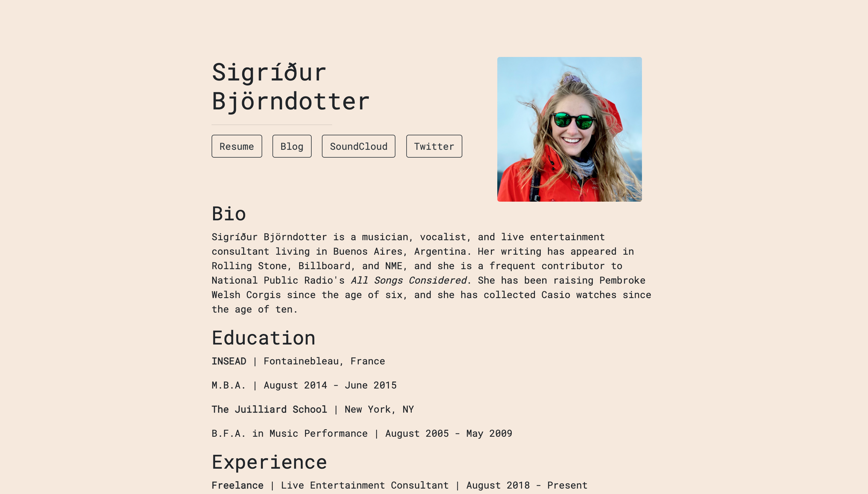
The postcards package makes it easy to create beautiful, single-page websites with minimal effort. It’s perfect for personal websites, portfolios, and project showcases. Using postcards allows you to present your work professionally and creatively, without needing extensive web development knowledge.

A collection of R Markdown templates for creating simple and easy-to-personalize single-page websites.

“The goal of the package is to make it easy for anyone to create a one-page personal website using an R Markdown document.”

Author: Sean Kross [aut, cre]
Maintainer: Sean Kross <sean at seankross.com>
https://CRAN.R-project.org/package=postcards
GitHub: https://github.com/seankross/postcards
Similar to https://pages.github.com/
Your webpage should say something about you, your interests, and your projects, as well as how to contact you.

Some examples:

14.5.1 Installation

In this case, the package is already installed.

## You can install Postcards with the following command:
# install.packages("postcards")

## Or you can install the latest development version (not recommended):
# remotes::install_github("seankross/postcards@main")

14.5.2 Templates

Postcards include five templates: Jolla, Jolla Blue, Trestles, Onofre, and Solana. Each site is optimized for viewing on both desktop and mobile devices. The goal of the package is to make it easy for anyone to create a one-page personal website using an R Markdown document.

Jolla:

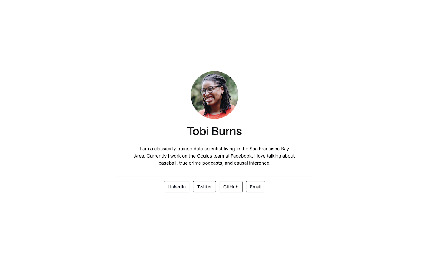
Jolla Blue:

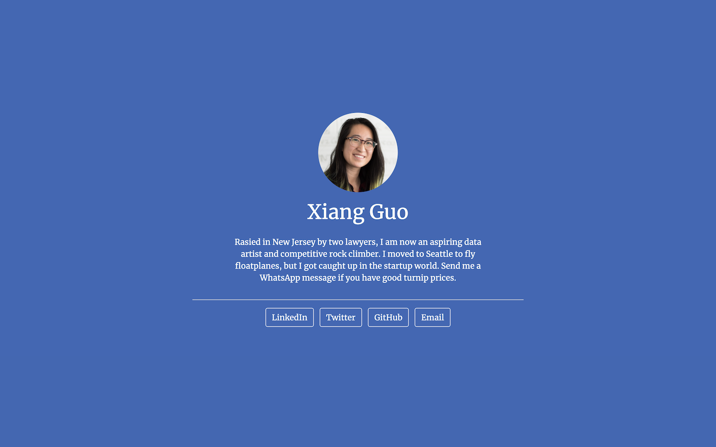
Trestles:

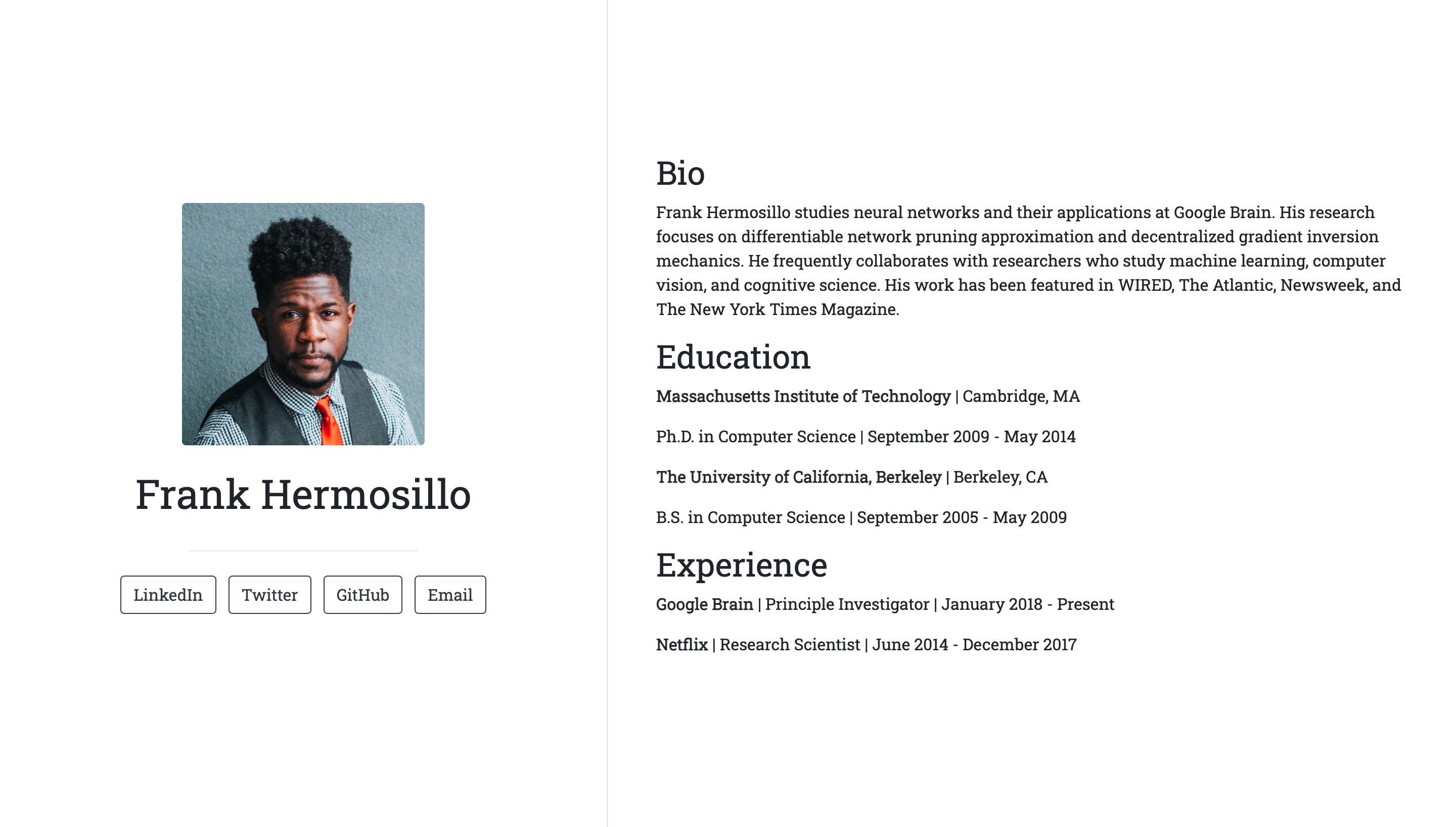
Onofre:

Solana:

To start personalizing one of these templates, you need to create a new project.

14.6 Create your own website with postcards!

https://www.youtube.com/watch?v=Q6eRD8Nyxfk&list=PLNNI62fcZPdB3G8Nl87gUlAQTEe2EH5K4&index=43

Create your own website:

Following the next steps you will be able to create your own personal website.

You will need to have a GitHub account and connect Git. In case you missed it, you can go back to the “Git + GitHub” section.

14.6.1 Create a New Project in RStudio (Interactive Selection)

If you use RStudio:

Select “File”, “New Project”…
Choose “New Directory”, “Postcards Website”
Enter a directory name for your project in RStudio (“Your_Username.github.io”)
Choose one of the templates from a dropdown menu

Select “Create Project” after choosing a name for the folder that will contain your site. This folder will contain two important files:

An R Markdown document with your site’s content
A sample photo you should replace (with your own)

## Create a new project
usethis::create_project("Your_Username.github.io")

14.6.2 Set Up Git and GitHub

To save changes, you need to set up Git and GitHub

## Set up Git and GitHub
usethis::use_git() # Restart the session
usethis::use_github()

14.6.3 Choose a Template

## Choose only one template (the one you like the most)
postcards::create_postcard(template = "jolla")
postcards::create_postcard(template = "jolla-blue")
postcards::create_postcard(template = "trestles")
postcards::create_postcard(template = "onofre")
postcards::create_postcard(template = "solana")

In this way, you will also get the 2 important files:

An R Markdown document with your site’s content
A sample photo you should replace

14.6.4 Edit with Your Information

Now you should edit the R Markdown document with your information and replace the image with one of your choice :)

Fill in your information using the Markdown format. For example, https://github.com/andrewejaffe/andrewejaffe.github.io/blob/master/index.Rmd#L17-L31.

Add your profiles in the style of https://github.com/andrewejaffe/andrewejaffe.github.io/blob/master/index.Rmd#L7-L12

14.6.5 Deploy the Page

To compile the self-contained HTML file for the site:

In RStudio, you can use the “Knit” button or directly:

## Deploy the GitHub page
rmarkdown::render("index.Rmd")