6 Interpreting model coefficients with ExploreModelMatrix

Instructor: Leo

6.1 Model objects in R

Linear regression review https://lcolladotor.github.io/bioc_team_ds/helping-others.html#linear-regression-example
With R, we use the model.matrix() to build regression models using the Y ~ X1 + X2 formula syntax as exemplified below.

## ?model.matrix
mat <- with(trees, model.matrix(log(Volume) ~ log(Height) + log(Girth)))
mat
#>    (Intercept) log(Height) log(Girth)
#> 1            1    4.248495   2.116256
#> 2            1    4.174387   2.151762
#> 3            1    4.143135   2.174752
#> 4            1    4.276666   2.351375
#> 5            1    4.394449   2.370244
#> 6            1    4.418841   2.379546
#> 7            1    4.189655   2.397895
#> 8            1    4.317488   2.397895
#> 9            1    4.382027   2.406945
#> 10           1    4.317488   2.415914
#> 11           1    4.369448   2.424803
#> 12           1    4.330733   2.433613
#> 13           1    4.330733   2.433613
#> 14           1    4.234107   2.459589
#> 15           1    4.317488   2.484907
#> 16           1    4.304065   2.557227
#>  [ reached getOption("max.print") -- omitted 15 rows ]
#> attr(,"assign")
#> [1] 0 1 2

colnames(mat)
#> [1] "(Intercept)" "log(Height)" "log(Girth)"

How do we interpret the columns of our model matrix mat?

summary(lm(log(Volume) ~ log(Height) + log(Girth), data = trees))
#> 
#> Call:
#> lm(formula = log(Volume) ~ log(Height) + log(Girth), data = trees)
#> 
#> Residuals:
#>       Min        1Q    Median        3Q       Max 
#> -0.168561 -0.048488  0.002431  0.063637  0.129223 
#> 
#> Coefficients:
#>             Estimate Std. Error t value Pr(>|t|)    
#> (Intercept) -6.63162    0.79979  -8.292 5.06e-09 ***
#> log(Height)  1.11712    0.20444   5.464 7.81e-06 ***
#> log(Girth)   1.98265    0.07501  26.432  < 2e-16 ***
#> ---
#> Signif. codes:  0 '***' 0.001 '**' 0.01 '*' 0.05 '.' 0.1 ' ' 1
#> 
#> Residual standard error: 0.08139 on 28 degrees of freedom
#> Multiple R-squared:  0.9777, Adjusted R-squared:  0.9761 
#> F-statistic: 613.2 on 2 and 28 DF,  p-value: < 2.2e-16

6.2 ExploreModelMatrix

It’s a Bioconductor package which is useful to understand statistical models we use in differential expression analyses. It is interactive and helps us by creating some visual aids.
- http://www.bioconductor.org/packages/ExploreModelMatrix
For more details, check their paper https://doi.org/10.12688/f1000research.24187.2.
We’ll go over the examples they provide at http://www.bioconductor.org/packages/release/bioc/vignettes/ExploreModelMatrix/inst/doc/ExploreModelMatrix.html

6.3 Example 1

## Load ExploreModelMatrix
library("ExploreModelMatrix")

## Example data
(sampleData <- data.frame(
    genotype = rep(c("A", "B"), each = 4),
    treatment = rep(c("ctrl", "trt"), 4)
))
#>   genotype treatment
#> 1        A      ctrl
#> 2        A       trt
#> 3        A      ctrl
#> 4        A       trt
#> 5        B      ctrl
#> 6        B       trt
#> 7        B      ctrl
#> 8        B       trt


## Let's make the visual aids provided by ExploreModelMatrix
vd <- ExploreModelMatrix::VisualizeDesign(
    sampleData = sampleData,
    designFormula = ~ genotype + treatment,
    textSizeFitted = 4
)

## Now lets plot these images
cowplot::plot_grid(plotlist = vd$plotlist)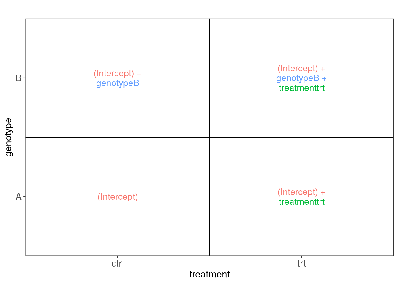

Interactively, we can run the following code:

## We are using shiny again here
app <- ExploreModelMatrix(
    sampleData = sampleData,
    designFormula = ~ genotype + treatment
)
if (interactive()) shiny::runApp(app)

6.4 Example 2

http://bioconductor.org/packages/release/bioc/vignettes/ExploreModelMatrix/inst/doc/ExploreModelMatrix.html#example-2

6.5 Example 3

http://bioconductor.org/packages/release/bioc/vignettes/ExploreModelMatrix/inst/doc/ExploreModelMatrix.html#example-3

6.6 Exercise

Exercise 1: Interpret ResponseResistant.Treatmentpre from the second example. It could be useful to take a screenshot and to draw some annotations on it.

Exercise 2: Whis is the 0 important at the beginning of the formula in the third example?

6.7 To learn more

A guide to creating design matrices for gene expression experiments:

“Model matrix not full rank”

http://bioconductor.org/packages/release/bioc/vignettes/DESeq2/inst/doc/DESeq2.html#model-matrix-not-full-rank

6.8 Community

Some of the ExploreModelMatrix authors:

Some of the edgeR and limma authors: